Asperity Contact Polynomial Coefficients
The asperity contact polynomial serves to establish a smooth transition between the hydrodynamic lubrication regime and the mixed lubrication regime for a Reynolds film. In the instances where the Reynolds film fails to bear the external loads, metal to metal contact on the asperity level can occur. Therefore, the polynomial-based contact model ensures a smooth transition between the instances of full film operation and asperity contact-based operation. In typical positive displacement machines, such asperity contact is common during start-up and high load-low speed operation.
Steps to Generate Asperity Contact Polynomial
There is a MATLAB script named asperityFit.m in the Utilities, which can be utilized to generate the asperity polynomial coefficients required as inputs to the ReynoldsFilm::assignAsperityPolyFit() contact model. It requires user input for specific material properties and surface roughness of both the lubricating interfaces.
Required user input: User needs to provide the the Young’s modulus, yield strength, Poisson’s ratio of both the bodies forming the lubricating interface.
Running the MATLAB script, non-dimensional hardness or
NDHardwill be calculated using the following equation [LeeRen1996]:\(NDHard = \frac{2*3*{\sigma}*{ACL}}{{\pi}*{E_{eq}}*{Rg}}\)
Where \(\sigma\) is the equivalent yield stress, \(ACL\) is the autocorrelation length, \(E_{eq}\) is the equivalent Young’s modulus, and \(Rq\) is the equivalent roughness. The lowest value of the yield strength is considered as the equivalent yield strength, The equivalent Young’s modulus and equivalent roughness are calculated using the formula mentioned in [LeeRen1996].
The same MATLAB script with calculated
NDHardwill interpolate the non-dimensional contact pressurePCwith the help of non-dimensional average gap and non dimensional hardness.Utilize the Curve Fitting Toolbox in MATLAB to fit a curve between the variables
PCandlnHon \(y\)-axis and \(x\)-axis, respectively, with the \(R^2\) close to 1. \(R^2\) is a statistical measure used to assess how well a regression model fits the data, essentially indicating the proportion of variation in the dependent variable that can be explained by the independent variable(s) in the model; the higher the \(R^2\) value (between 0 and 1), the better the model fits the data, with 1 representing a perfect fit. The following image illustrates an example seventh-degree polynomial fit:
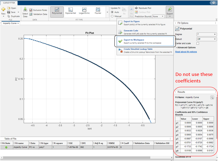
Export the fitted polynomial in the workspace to get the correct value of the coefficients. Do not copy paste the coefficients value from the results (Bottom right corner in the above figure). A little change in decimal place of the coefficients can leads to a completely different polynomial line.
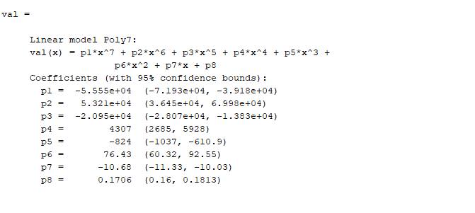
As long as the polynomial curve fits well with the data points, the coefficients are good to use, irrespective of the polynomial order. Higher the order of the polynomial, more sensitive the coefficients are. Therefore, it is suggested to use them very carefully.
Using Asperity Contact Polynomial in Multics
In order to utilize the asperity contact polynomial for a Reynolds film, the ReynoldsFilm::assignAsperityPolyFit() method needs to called in the main sketch. An example of how to call this method is shown below:
blockFilm.assignAsperityPolyFit(dictInOut.readArray("polyCoeffsBlockFilm", uNone));
The corresponding entry in the inputDict.txt should be as follows (where p1, p2, …, p10 are replaced by the values generated by MATLAB above):
polyCoeffsBlockFilm - [p1; p2; p3; p4; p5; p6; p7; p8; p9; p10]
It is not mandatory to have 10 coefficients. Depending on the order of polynomial, the number of coefficients should be provided. For example, 4th, 7th and 9th order polynomials will have 5, 8, and 10 coefficients respectively.