External Gear Machine
This tutorial is for modeling external gear machines (EGMs).
What is an External Gear Pump?
An external gear pump (EGP) is a type of EGM that moves fluid from a low pressure region to a high pressure region. Alternatively, an external gear motor is an EGM that moves fluid from high pressure to low pressure.
An EGP is a type of positive displacement pump that uses the trapped volume between the gear teeth and the casing, named the tooth space volume (TSV) to transfer fluid from an inlet to an outlet. Read this page to learn more about EGMs.
How to Simulate an EGM
First, we need to define the requirements for simulating an EGM and they are the following:
Geometry Generation
Gear Tooth Profile
Body STL Files
Geometry Input File
Polygons
Influence Matrix
Sketch Creation
inputDict Definition
Geometry Generation
In order to generate the complete geometry of the EGM, we need to make a few things. These are the gear tooth profiles, STL files, geometry input file, polygons, and influence matrix.
The gear tooth profiles, and the STL files are prerequisites for creating the geometry input file and polygons. The geometry input file and polygons are created with the geometry generator. Additionally, the influence matrix is generated with ANSYS.
Gear Tooth Profile
The first step in generating the geometry input file is creating the gear tooth profile. Currently, Multics supports involute gears and continuous contact gears, and the process to create the gear profiles for these two types of gears is different.
Involute Gear Profile
To generate the involute gear tooth profile, you must run the gear generator executable file. An executable file has been created by multics team which takes in the different tooth profile values (viz. no. of teeth, module, addendum, dedendum etc) and processes it to produce toothprofile.txt, which you can further use to carry out your simulations. Please reach out to the Multics team to obtain access to the executable file.
This file uses input parameters and outputs a toothProfile.txt. The input parameters are the same parameters used when machining the gears and these are usually provided by the EGM manufacturer.
Here is a list of the input parameters and a brief explanation:
z - Number of teeth
m - Gear module
x - Dimensionless cutter offset distance, AKA gear profile shift offset. The positive value means that the cutter is further from the gear.
alpha_cutter - cutter slope angle, same for coast and drive
h_a - vertical distance between cutter ref line and cutter root
h_d - vertical distance between cutter ref line and cutter tip
r_fillet - cutter tip radius of fillet
CRmin - allowable minimal Contact Ratio
The first step with the geometry generation is to determine the minimum interaxis value and the maximum interaxis value. The minimum can be determined by finding the dual flank contact interaxis value. The maximum interaxis value is found by taking the nominal interaxis and adding 2x the radial shaft clearance. Now that you know the maximum and minimum interaxis for the pump, you need to choose 3 other interaxis values that are between the max and min (for a total of 5). These must be linearly spaced values.
Continuum Gear Profile
To create the tooth profile for continuous contact gears, you must use a MATLAB script, Arcgenerator.m. Reach out to the Multics team for access to this file. This script works similarly to the involute profile script as it takes user inputs and creates an output file called toothProfile.txt.
Here is a list of the input parameters and a brief explanation:
R - Pitch radius
Alpha - Pressure angle
z - Number of teeth
b - Center to center distance of the gears
Once you define the above input parameters, you can run the MATLAB script. For more details about how the gear profile is calculated refer to Source [1] and Source [2].
STL Creation
The next step in the geometry process is the generation of STL files. If the top and bottom bearing blocks are symmetric then you will need 5 STL files, otherwise you will need 8. Here is a list of the STL files needed:
Casing
Bearing Block
Suction Groove (Top and Bottom if asymmetric. Top if symmetric)
Delivery Groove (Top and Bottom if asymmetric. Top if symmetric)
Backflow Groove (Top and Bottom if asymmetric. Top if symmetric)
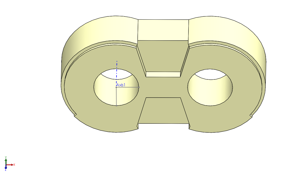
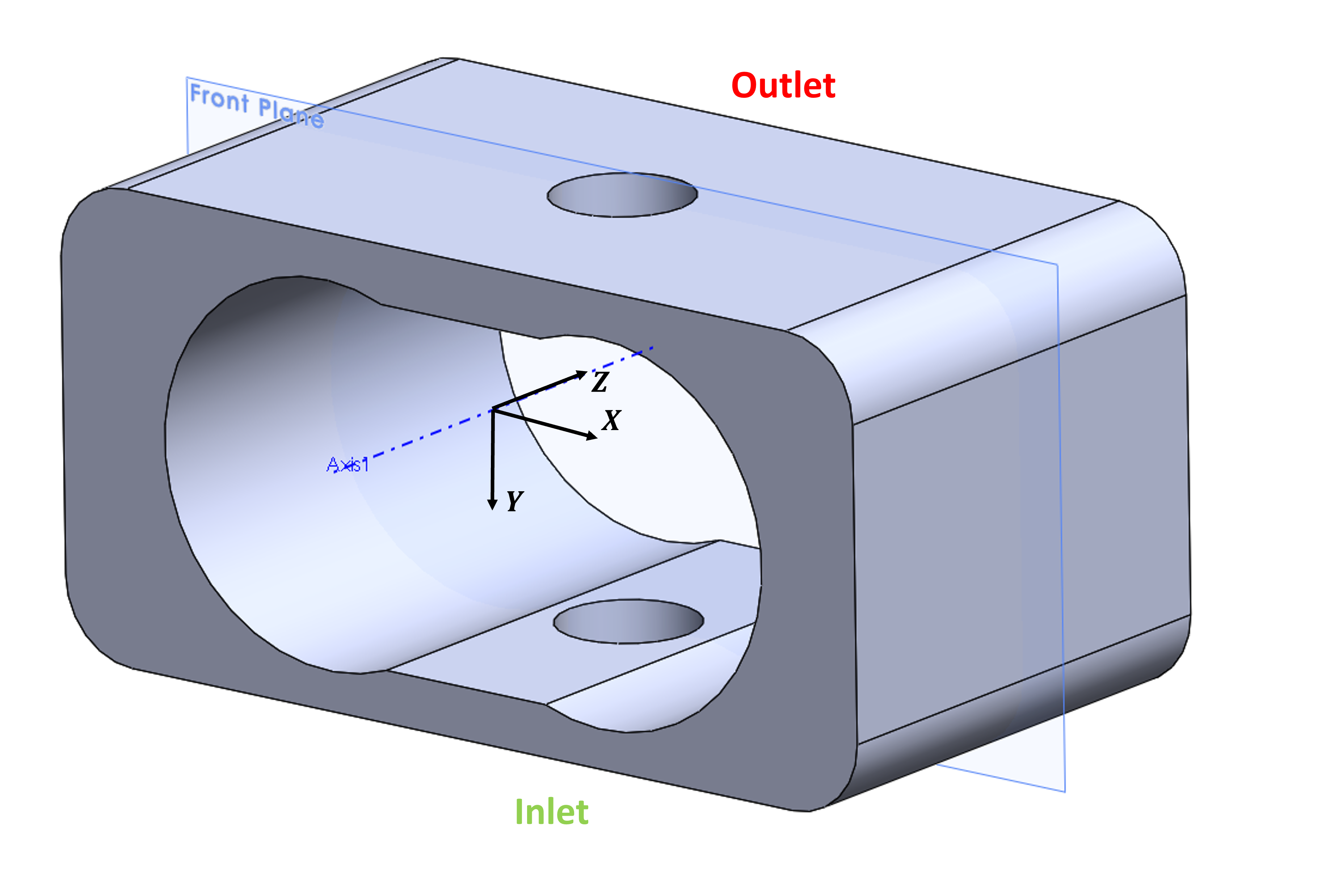
These files are generated with the 3D model of the bearing block. First, you need to create a Solidworks assembly file and include the bearing block part, a (.sldprt) file to the assembly. Now, you should make this bearing block float by rick-clicking the bearing block and clicking “float”. This unconstrains the bearing block. Next, you are going to want to draw 3D sketch lines on the bearing block in the .sldprt file. You need to draw 3 lines that intersect at the center of the drive gear bearing, and these 3 lines are all orthogonal. It does not matter how long these lines are. These lines are going to be used to position the object in the assembly space and the lines are shown in the following image.
Now go back to the assembly, and mate the intersecting point coincident with the origin of the assembly. Next, mate the axes with the locating lines so that the bearing block is fixed in space in the following orientation.
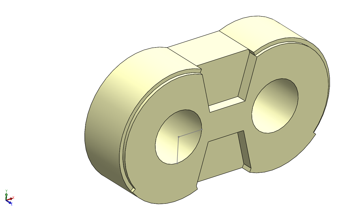
This orientation is the same as the standard orientation which is obtained by placing the drive side on the left (-x), the inlet on the bottom (-y), and the outlet on the top (+y).
Now is a good point to save, and you are now ready to create the STL files. First, we are going to make the backflow grooves, and the process for this is exactly the same for creating the suction (inlet groove) and delivery (outlet groove) STL files.
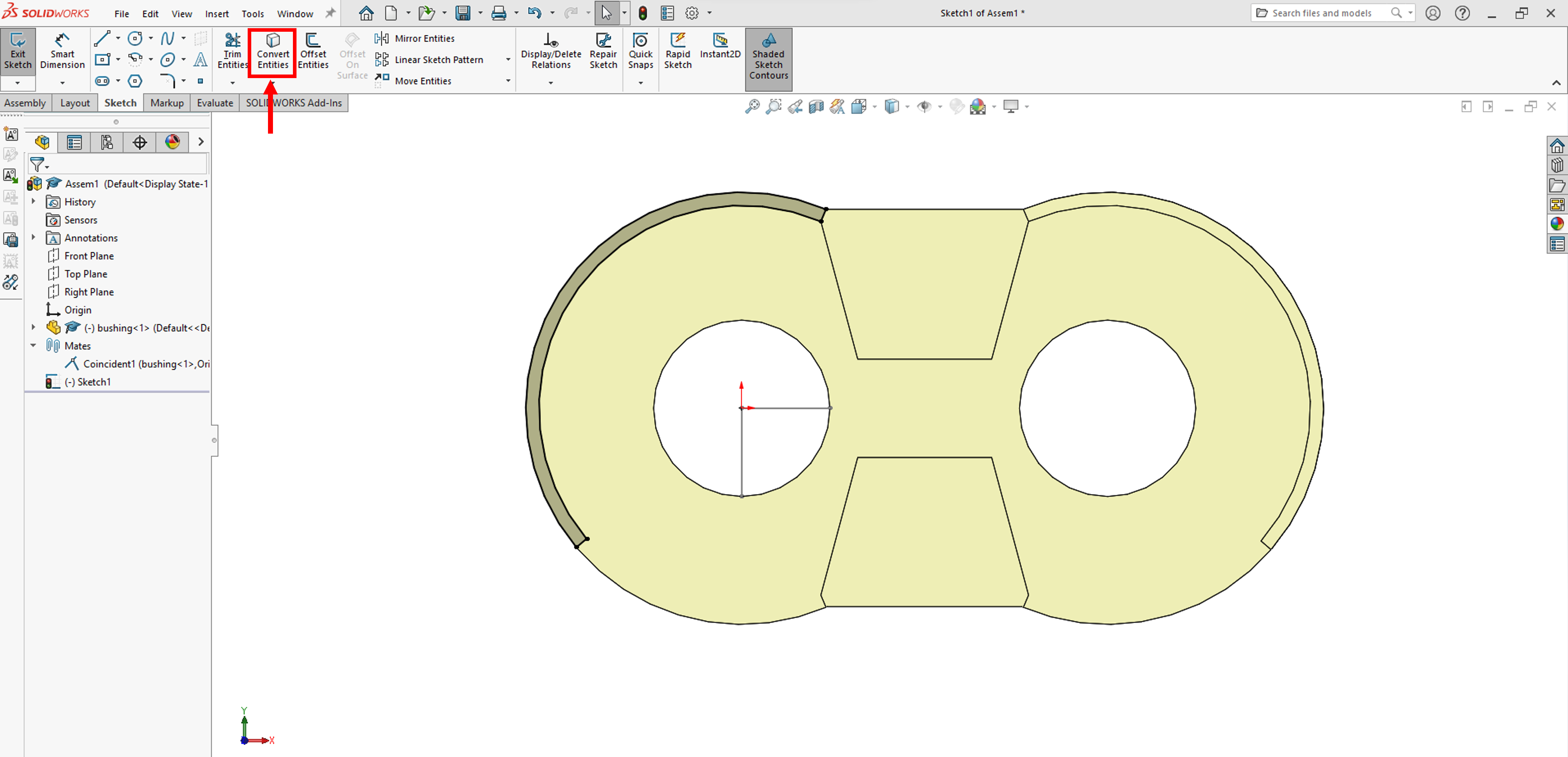
Click the create a new sketch button and select the face of the part that is closest to you as the plane to create your sketch on.
Next, you want to click on the face that is the drive side backflow groove, and then click “Convert Entities”. This creates a sketch of the backflow groove shape.
Note
You only need to do this for the drive side backflow groove.
Note
Sometimes, additional trimming operation must be carried out so that the entire backflow groove is obtained for STL generation.
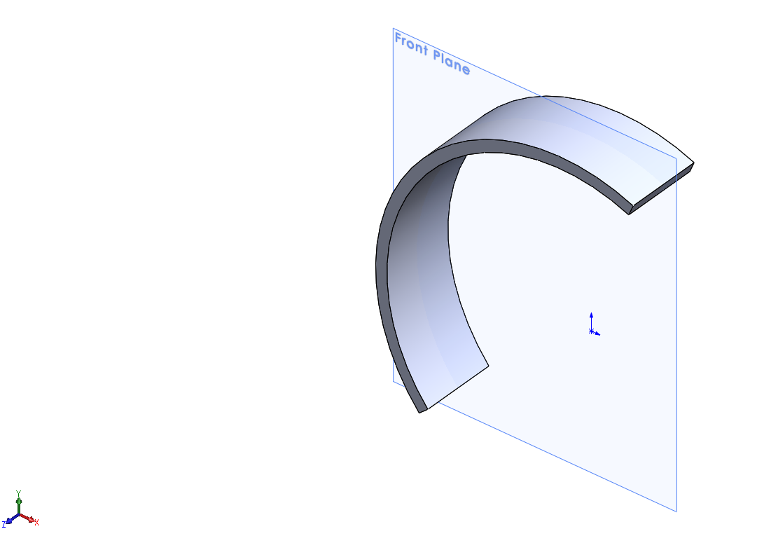
Now that you have an outline of the backflow groove you need to convert this closed sketch to a block. Select all the backflow groove sketch entities, right click on the selection, and click “make block”. If this is not an option on your right click menu you can go to Tools -> Block -> Make Block. Now that you have a block, save the block, and then open the block file.
In the block file, the next step is to extrude the block sketch by 10 mm and select “Mid Plane” as the direction. The end result will look like the following image.
Warning
It is CRITICAL that the block intersects the XY Plane.
Next, go to File -> Save As -> STL, and then click on “Options”. Change the output to “ASCII”, use millimeters as your unit, and adjust the resolution to your liking.
Warning
It is CRITICAL that you check the box that says “Do not translate STL output date to positive space”.
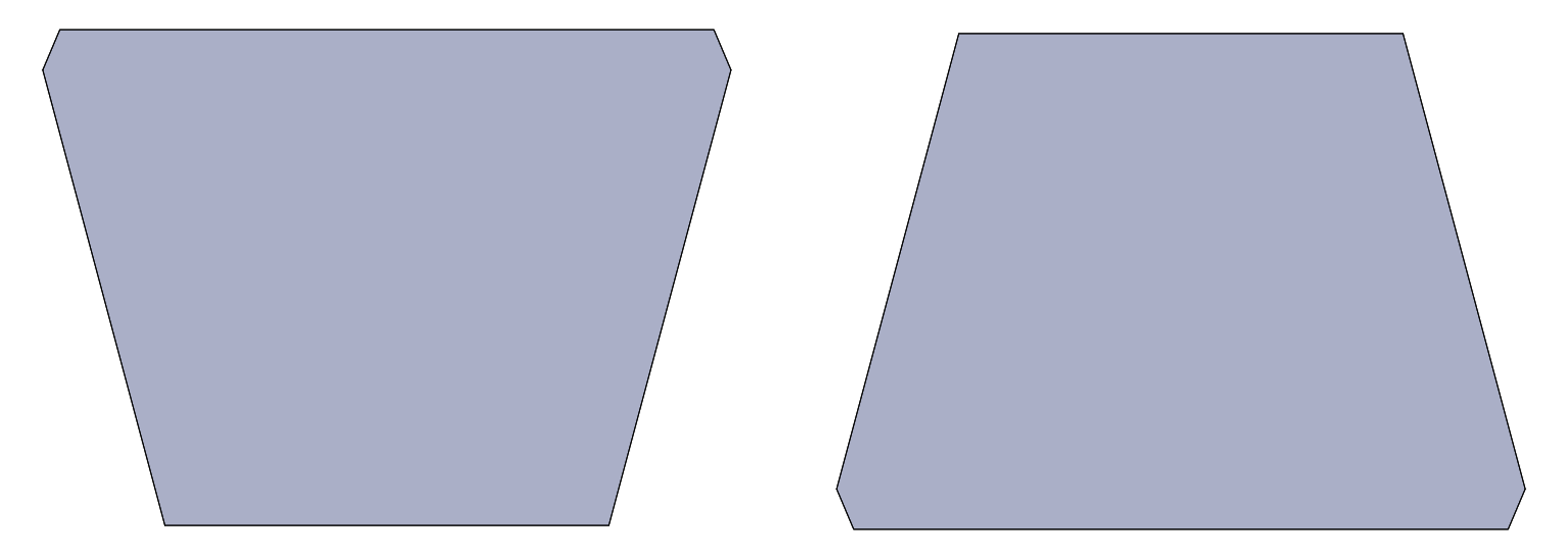
Now apply all those option changes and click save. These steps can be repeated for the suction and delivery groove which should look similar to this, where the left one is the suction groove and the right one is the delivery.
Finally, the bearing block STL file is made by creating blocks from the outside edges of the bearing block, and the casing STL file is simply a copy of the bearing block STL file. These would look like the following image, and should also intersect the XY plane.
Geometry Input file
Now in order for the software to understand the geometry, we must convert the toothprofiles, and STL files into the geometry input file which is done with the EG geometry generator. To obtain the files for the EG geometry generator reach out to the Multics team.
Navigate to the “Geometry” folder that has geometry.exe in it. Next create the 5 subfolders that are named the 5 different interaxis values. An example is a folder named “32.100”. These subfolders need to contain the the toothprofile.txt files that correspond to the interaxis value of the folder name. Additionally, the folders need to contain STLdirectory.txt, Inputdata.txt, and AdvancedSettings.txt. The STLdirectory.txt file should be the same for all the different interaxis folders, and this file simply tells the geometry generator the names of the necessary STL files. So update this file to match your STL files, and place your STL files in the referenced folder.
Next, the Inputdata.txt file needs to be changed to match the EGM geometry. Here is a list of the required inputs and what they mean.
- Teeth Number [Integer]
Number of teeth on the gear
- Interaxis [mm]
Distance between the gear shafts for the respective
toothprofile.txt- Gear’s Whole Depth [mm]
Thickness of the gear, not to be confused with the tooth depth.
- Minimum Contact Clearance [mm]
BLANK
- Save graphic files [TXT/VTK/N/POLY]
Type of graphical geometry file to output
TXT - TXT based graphical file used for debugging
VTK - VTK based graphical file used for debugging
N - No
POLY - Polygon file used in simulation to solve lateral gap film
- Delta Angle [deg]
Angular difference between drive and driven gear tooth space volume locations. The default value can be zero as the calculation of delta angle is done by the geometry code using the generated tooth profile.
- Number of Calculation Steps for Each TSV [Integer]
Number of saved data points for every nth gear tooth. A value of 300 for a 12 tooth gear creates a 3600 column table.
- Groove Option [0/1/2/3]
Option to give the input about relief and back flow grooves
0 - No groove
1 - Full parametric grooves
2 - Using STL files (Use this option in case the design of grooves is already evaluated and STL files are generated as outlined above.)
3 - Rectangular parametric grooves
- Hole on the Groove [Y/N]
Option to check if the grooves have through holes. In most cases this option should be N.
- Helical Rotation Angle [deg]
Angle of gear helical rotation
- Advanced Mode [Y/N]
Activates the
AdvancedSettings.txtfile. Most of the time this should be Y.
The values that should be changed between all the interaxis folders should just be the interaxis value, and the delta angle. Once this is done, open up AdvancedSettings.txt, which takes the following inputs.
- Matching the Groove to Bearing Block [Y/N]
If yes, the code identifies where the groove belongs on the bearing block rather than basing it off of the coordinates of the STL file.
- Starting Point of Working Profile [mm]
BLANK
- Angle tolerance
Tolerance for tooth profile angular span. User is recommended to use the default value unless issues are seen in generated geometry table.
- Figure Saving Frequency [Integer]
Saves a figure every n frames. The total frames per revolution is the column count of geometry table.
- Calculate 3D Force Feature [Y/N]
Flag determining if 3D force feature should be calculated.
- Profile Contact Ratio [-]
Gear contact ratio - average number of gear teeth meshing together during operation.
- Base Circle Radius [mm]
Gear base circle radius
- Groove Shift in Y-Direction [mm]
Assign shift of grooves in Y-direction
- Force Calculation Option [0/1/2]
0 - Complete, fully 3D
1 - Only 2D -
for debugging2 - 3D from 2D file -
for debugging
- Casing Opening Angle When no Groove [deg]
Angle at which casing opens to tooth space volumes without presence of any grooves.
- Shaft Radius [mm]
Radius of gear shafts
- Continuum Modeling [Y/N]
Flag notifying whether gears are continuous contact gears.
- Relief Groove Option [0/1/2]
0 - Only one side
1 - Two symmetric sides
2 - Two asymmetric sides
- Writing File Unit Change [Y/N]
Change units of
AdvancedSettings.txtfile.- Averaging the EHL features (only for helical gears) [Y/N]
Flag to average EHL features for helical gears.
In the AdvancedSettings.txt file you only need to change the profile contact ratio, and the base circle radius for each of the 5 interaxis values. If you are using a continuous contact gear profile, make sure to change the Continuum Modeling flag in the AdvancedSettings.txt
Once your input files are all properly configured, run the file called runGeom.bat. This will create a geometry file in each interaxis folder, and finally these need to be combined so then run runCombine.bat.
Finally, if you want to use Reynolds films, you need to create polygon files. This only needs to be done once per pump rather than once per interaxis. In order to do this, create an a folder called output in one of the interaxis sub folders. Next run the runGeom.bat, and this will output polygon files into the output subfolder. All polygon files except the snapping polygons are generated by the geometry code run.
To generate snapping polygons, open MATLAB and navigate to /Utilities relative to the Multics installation directory. Open the file called make_polygon_series_from_tooth.m, give it the proper file paths and run it.
The user required inputs are shown below.
make_polygon_series_from_tooth.m1#Delta angle between drive and slave gears
2deltaAngle=17.691042;
3
4inp=read_inputDict('<PATH TO THE inputDict.txt File of the simulation>');
5toothpath='<PATH TO THE toothprofile.txt file used for geometry code generation>';
6geomoutpath='<PATH TO THE output folder where polygon files mentioned above are written>';
7newfilepath='<PATH TO THE FOLDER where snapper polygon files must be written>';
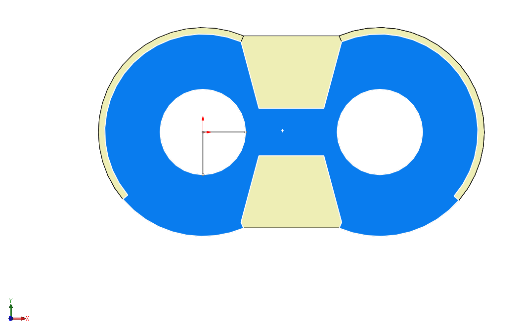
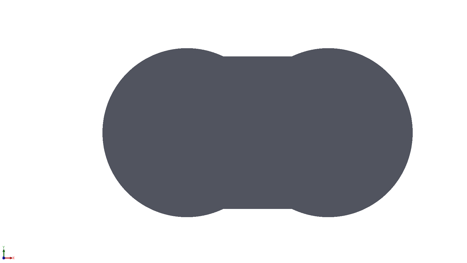
For modeling casing bushing films, corresponding boundary conditions shown in the figure below are assigned with fixed polygons. For generating the polygons, x and y coordinates of the corresponding grooves must be determined from the CAD file. It is important to make sure that the location of initial and final point in the polygon file is the same. Example polygons files can be found in the Polygons subfolder. To visualize the polygon files, open MATLAB and navigate to /Utilities relative to the Multics installation directory and open the file called polygonseries_viewer.m
Influence Matrix
Influence matrix is used by Multics to evaluate deformation of floating bodies and use the deformation information in lubricating interface calculations. In external gear machines, the deformation of lateral bushings or plates can be evaluated using influence matrix approach. The influence matrix is generated by an in house software called Influgen. The process of generation of influence matrix for a lateral bushing can be found in the Influgen documentation.
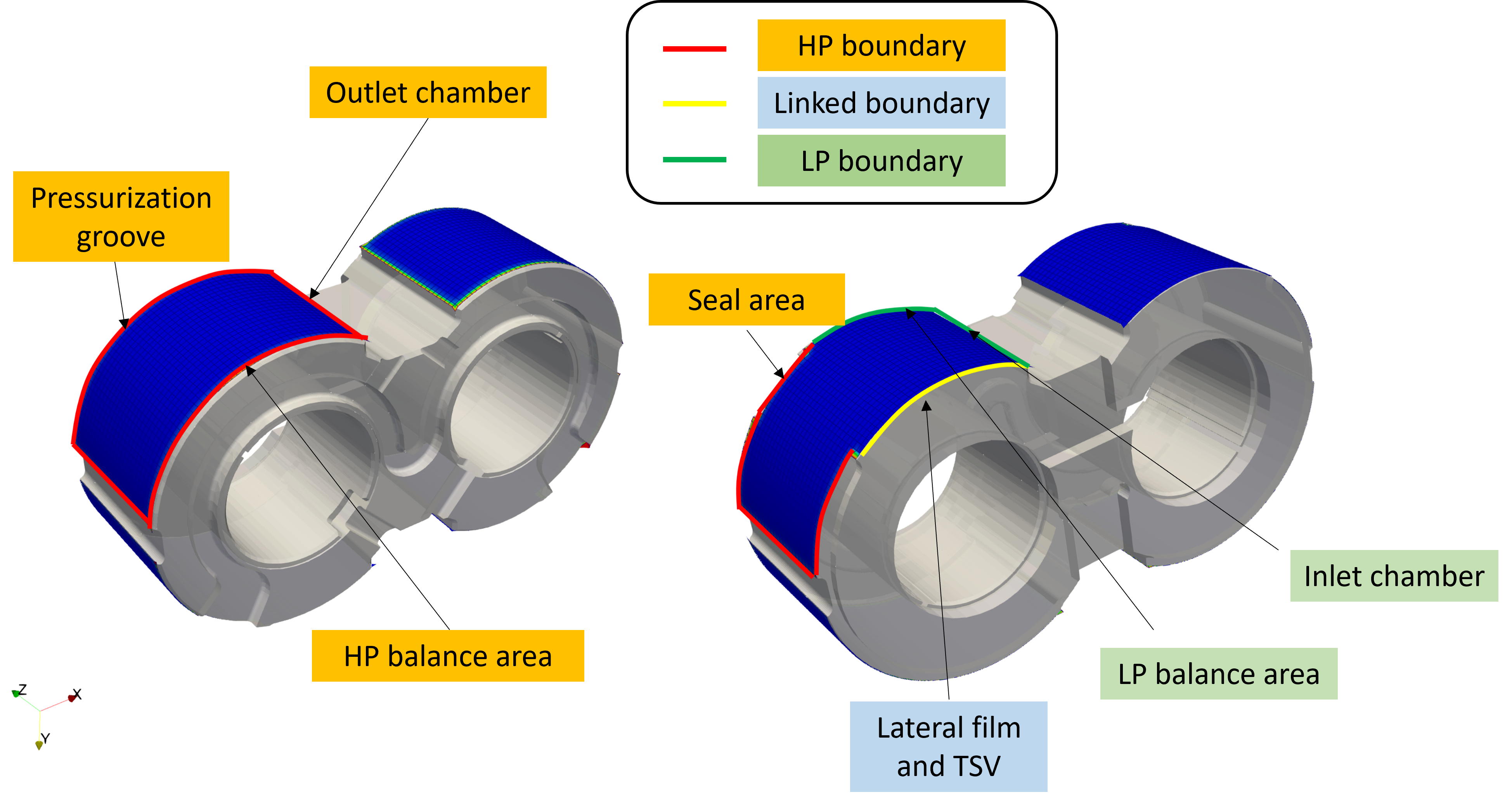
For the case of external gear machine, the deformation of the lateral bushing can be calculated using influence matrix method. Brief details of what areas must be selected for different named selections are provided here.
The figure below shows the required named selection assignments for the influence matrix generation of lateral bushing. Additionally, corresponding balance side areas at low or high pressure must be added to either to inlet or outlet named selection respectively.
Coordinate System
This section describes coordinate systems followed by the external gear machine simulation model in Multics. There are two types of coordinate systems generally defined in Multics which are global and body coordinate systems.
Global Coordinate System
The global coordinate system is defined as shown in the figure below. The global origin is defined at the drive side casing cavity center in both planar as well as axial sense. The \(x\) axis is defined by the line joining the drive side casing cavity center to the driven side casing cavity center with positive direction pointing from drive side to driven side. The positive \(y\) axis points towards the inlet port side. The positive \(z\) axis is decided using the right hand rule. The axial direction in which positive \(z\) axis points is referred to as Bottom side while the axially opposite side is referred to as Top side. Thus the positive \(z\) axis points from Top to Bottom side.
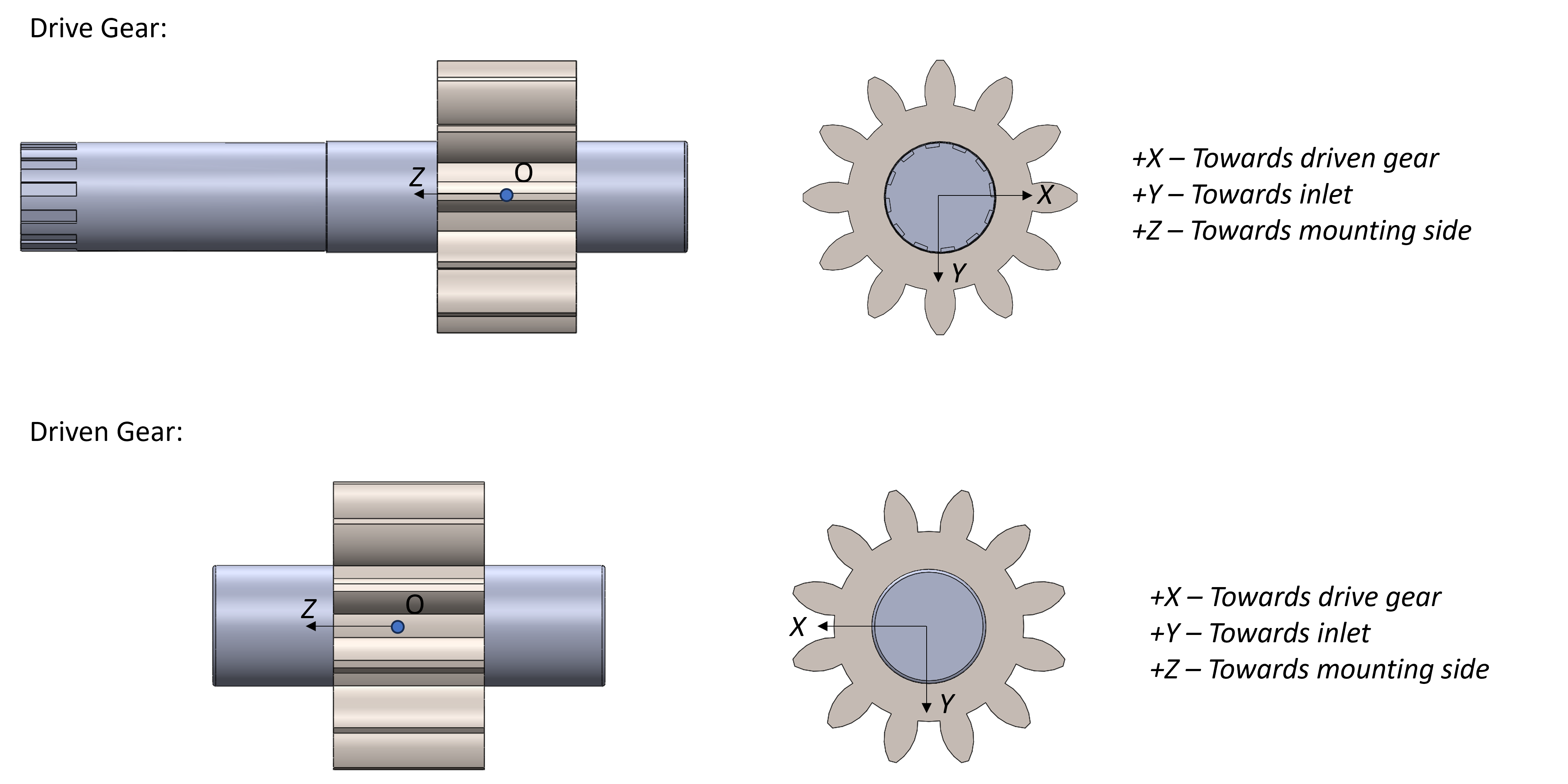
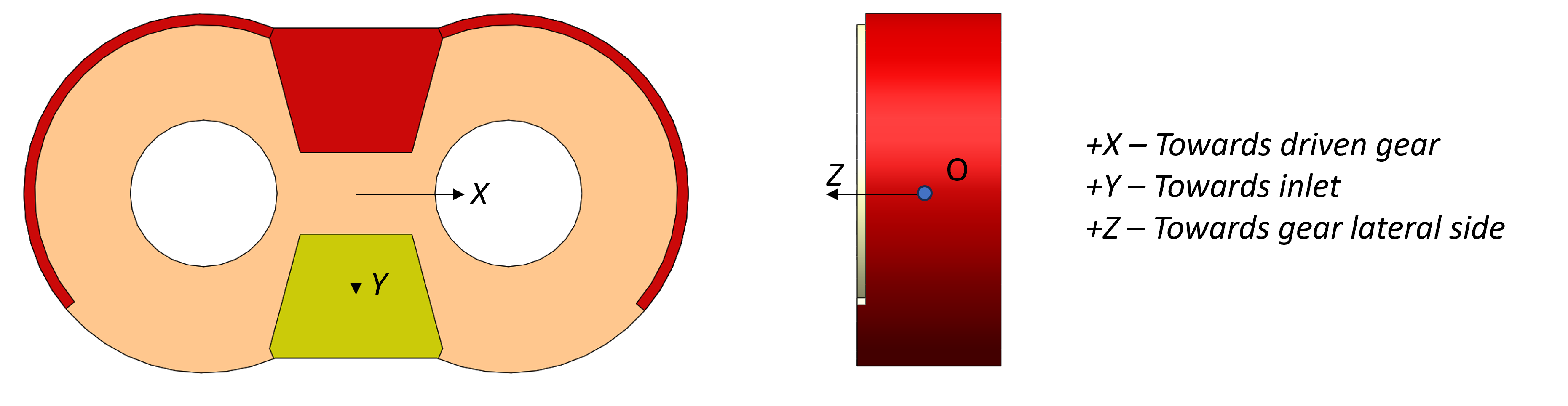
Body Coordinate Systems
The three main bodies involved in an external gear machine simulation are drive gear, driven gear and lateral bushing. The body coordinate systems for these bodies are shown in the figure below.
Lateral Balancing Mechanisms
In external gear machines, lubricating films are present on the lateral side of the gears. To minimize leakages through this lubricating interface, lateral balancing mechanisms are employed. There are multiple options of lateral balancing.
No balancing component - In this case the lateral side gap height is controlled by manufacturing tolerances between the lateral side of gears and the casing body. This option can be preferred for low pressure operations while for high pressure operations a balancing component must be included.
Lateral bushing - Most pressure compensated external gear machines include lateral bushings as balancing mechanisms. The balance side of the bushings contain regions of high pressure which are used to compensate the forces acting from the gear side on the plate and minimize the lateral gap height to reduce leakages. The journal bearings are also housed in the lateral bushing in this case.
Lateral plates - Some EGMs use lateral plates instead of bushings as balancing mechanisms. The difference compared to bushings is that the plates are thin and the journal bearings are generally housed in the casing in this case.
Casing Modeling Considerations
In modeling of external gear machines, accurate evaluation of leakages between the gear tip and the housing is important towards estimation of volumetric efficiency and TSV pressurization. Before normal operation of an external gear pump, the internal casing surface of the pump is worn in. This happens as gears exhibit motion from high pressure side to low pressure side due to clearances at journal bearings and forces acting from TSVs, leading to penetration of gear tips in the housing causing wear. This process is important to maintain sealing at the inlet side between high pressure and low pressure region.
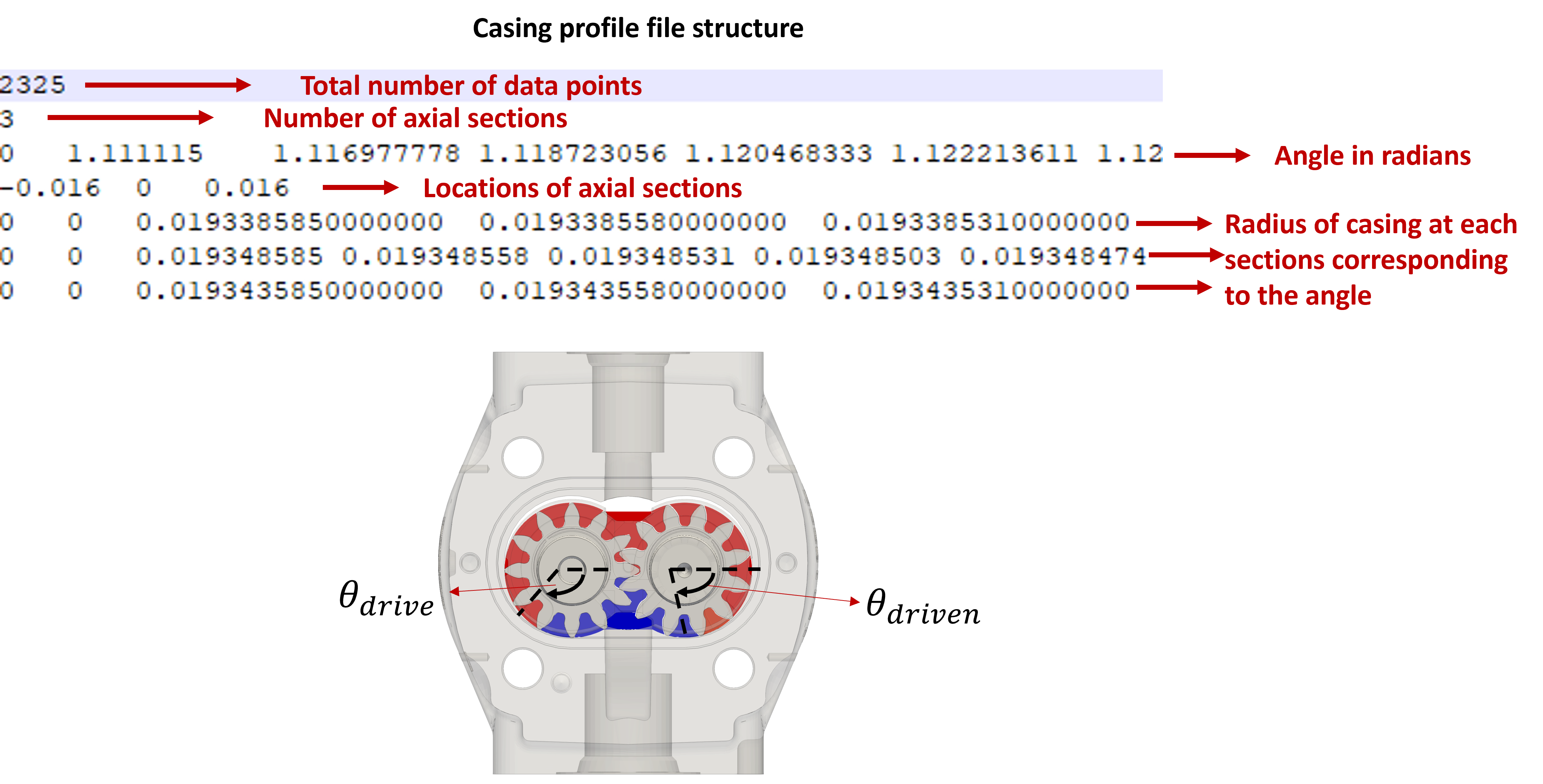
In Multics, the worn profile of the casing is generated via simulation and stored in a text file. It is also possible to measure the worn profile experimentally, and give it as an input to the simulation model. The input is given using text files, one each for drive and driven side profiles. It is also possible to measure as well as evaluate the worn profile at different axial sections and give it as an input to the simulation model.
Following image describes the structure of casing wear profile files for drive and driven gear.
The inputDict
The final step before you can simulate the EGP is to define variables in the inputDict. To see a completed list of necessary inputs and their explanations go to EGM inputDict Definition.
The simulation_results
External gear machine simulation allows visualization of various output parameters associated with different components of the machine. The simulation generates a outputlist.html file in the working folder. This file contains information regarding all output parameters that can be plotted. The variables that the user wants to visualize must be added to the simulation_results.txt file. As the simulation is running, the values of output variables with time will be written to the simulation_results.txt file which then can be visualized as detailed in the next section.
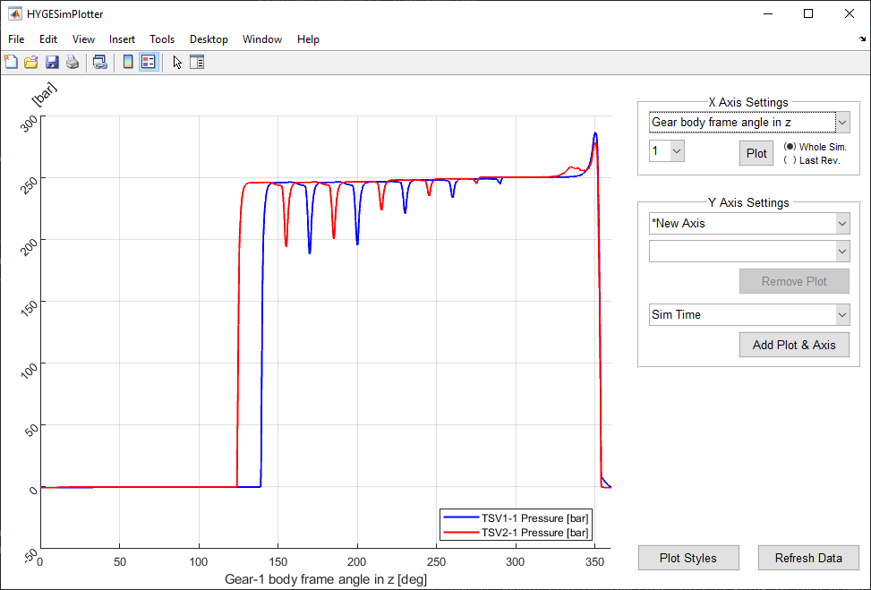
Analyzing Results
Once you have completed all the above steps, you can finally run Multics. Now in order to view the results, we need to navigate to the Multics installation directory and go to Utilities. Here there is going to be a file called MulticsPlotter.m, and you want to open MATLAB and add this to your working path. Once this is done type MulticsPlotter into the MATLAB console and it should find the function. This is going to then prompt you for a file, and you want to give it the simulation_results.txt. An additional feature of this plotter is that you can pass multiple simulation_results files to it, uniquely name them, and then compare the results. Once MATLAB loads the simulation_results file, you can then choose what variables you want on the X-axis and what variables you want on the Y-Axis. Here is an image of the plotted results for the example in Tutorials/External Gear Machine.