Axial Piston Machine

This tutorial is for modeling axial piston machines (APMs).

What is an Axial Piston Machine?

An axial piston machine (APM) is a positive displacement pump that displaces fluid based on the reciprocating motion of pistons within the bores of a cylinder block. For a swashplate-type APM, reciprocating motion is achieved with an inclined swashplate, which drives a number of pistons into and out of a cylinder bore which results in fluid displacement and suction respectively.

Multics-CASPAR is a Multics template designed for swashplate type axial piston pumps and motors.

Multics-CASPAR includes four core solvers, one for the lumped parameter calculation for chamber/port pressure and flow communication, and the rest three for each of the three lubricating interfaces. The options in Multics-CASPAR allows for running one core solver or multiples in a coupled fashion. It also allows for running with different variations. For example, the user can run only the lumped parameter analysis without any lubricating interfaces, or run a piston cylinder interface coupled with a slipper interface, or lumped parameter model coupled with one cylinder block interface, nine piston interfaces and nine slipper interfaces. The simulation options for the Multics-CASPAR template are defined in Simulation Options.

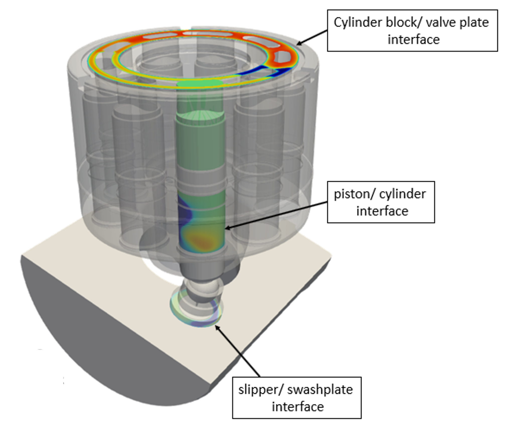
It can simulate energy/volumetric/torque efficiency, outlet/inlet/drain flow rate, flow ripples, forces, and moments applied on various moving bodies and bearing interfaces. It is also capable of providing insights into important aspects of swashplate machines, such as the pressure and flow rate of each individual displacement chamber, friction, leakage, and pressure distribution in lubricating interfaces considering full film lubrication or mixed lubrication, macro and micro motion of the moving bodies, solid body elastic deformations, fluid and solid domain temperature distributions and their effects in fluid behavior and solid deformation.

The tutorial documentation describes the steps involved in the simulation of the APM using a template class.

APM Modeling Concepts

APM Terminology

Coordinate System

Global Coordinate System

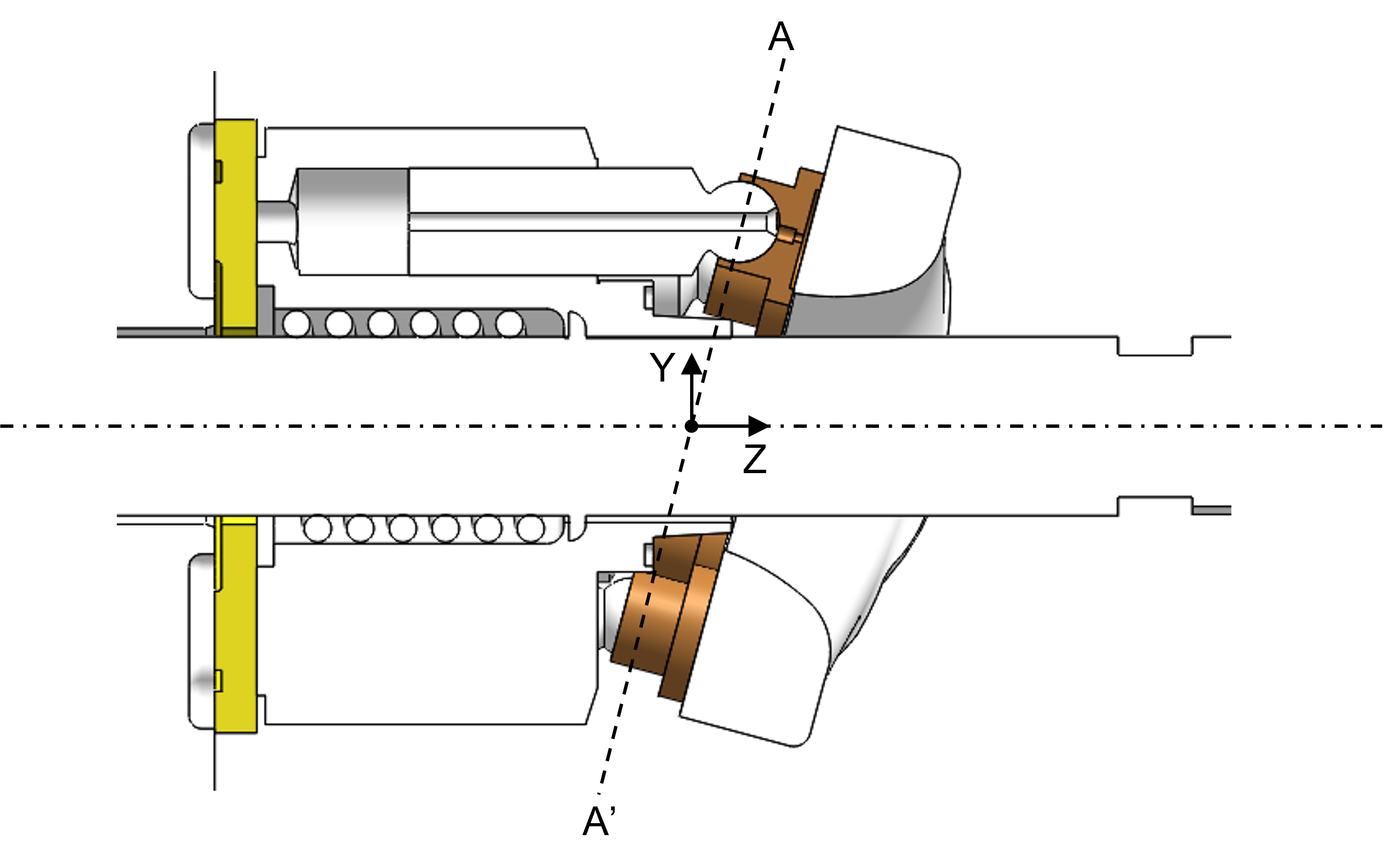
The global coordinate system is defined in the figure below. The global origin is defined as the intersection of the shaft axis and the plane (A-A’) through the piston ball joint centers. The \(+z\) axis points towards the swashplate. The \(x\) axis is defined as the axis about which the swashplate is swiveled. When the shaft rotation speed is counterclockwise about the \(+z\) axis, the \(+x\) axis points towards the outlet of the pump. The \(+y\) axis can be defined by right-hand rule.

Body Coordinate Systems

The body coordinate systems are required to specify key distances in the geometry of the APM. That said, the following description describes the initial state of the coordinate system when the simulation is initialized. The coordinate system and the origins of the body move with the body macro and micro-motion during the simulation.

Piston

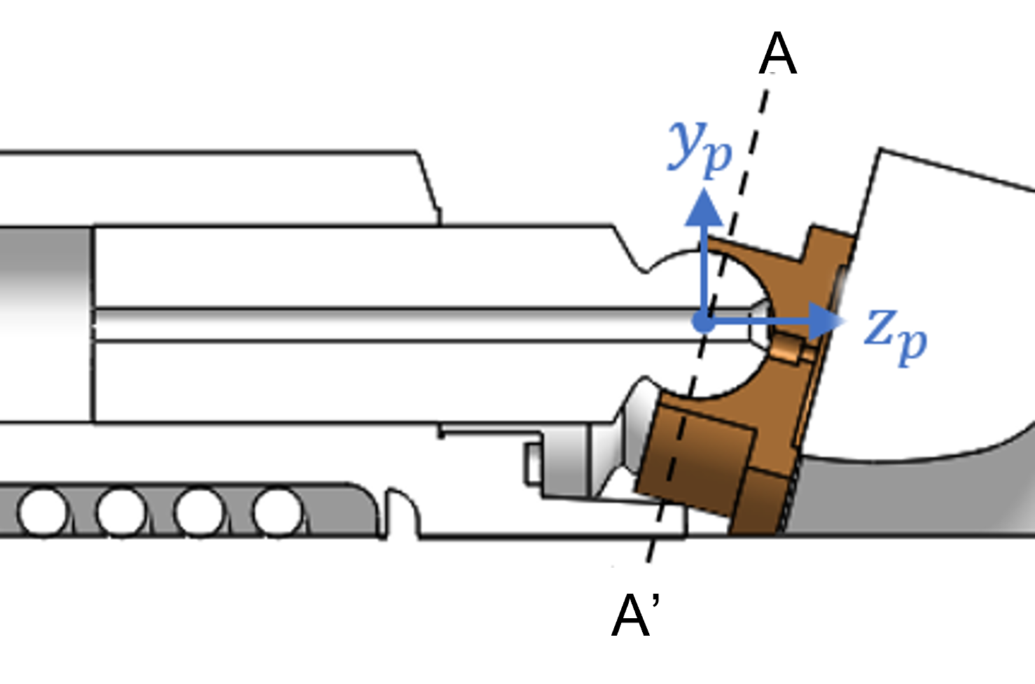
The piston body origin is defined at the ball joint center such that the \(+z\) axis points towards the swashplate parallel to the shaft axis. The other axis definitions are summarized in the figure below and follow the right-hand rule.

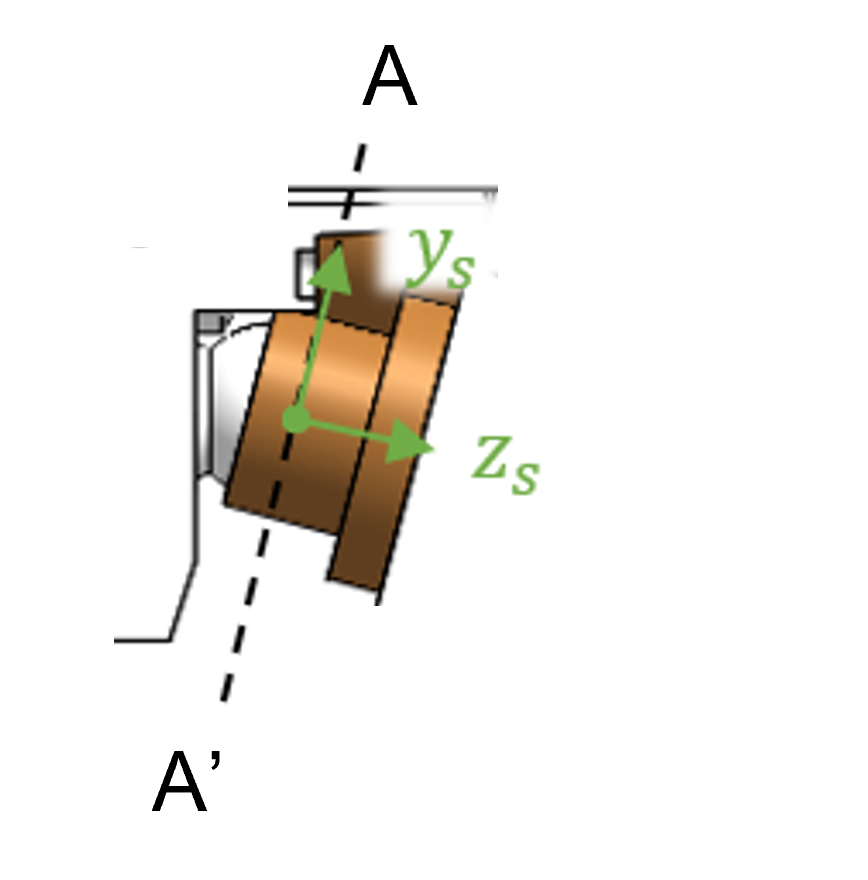
Slipper

The slipper body origin is defined at the ball joint center such that the \(+z\) axis points towards the swashplate normal to the swashplate running surface. The other axis definitions are summarized in the figure below and follow the right-hand rule.

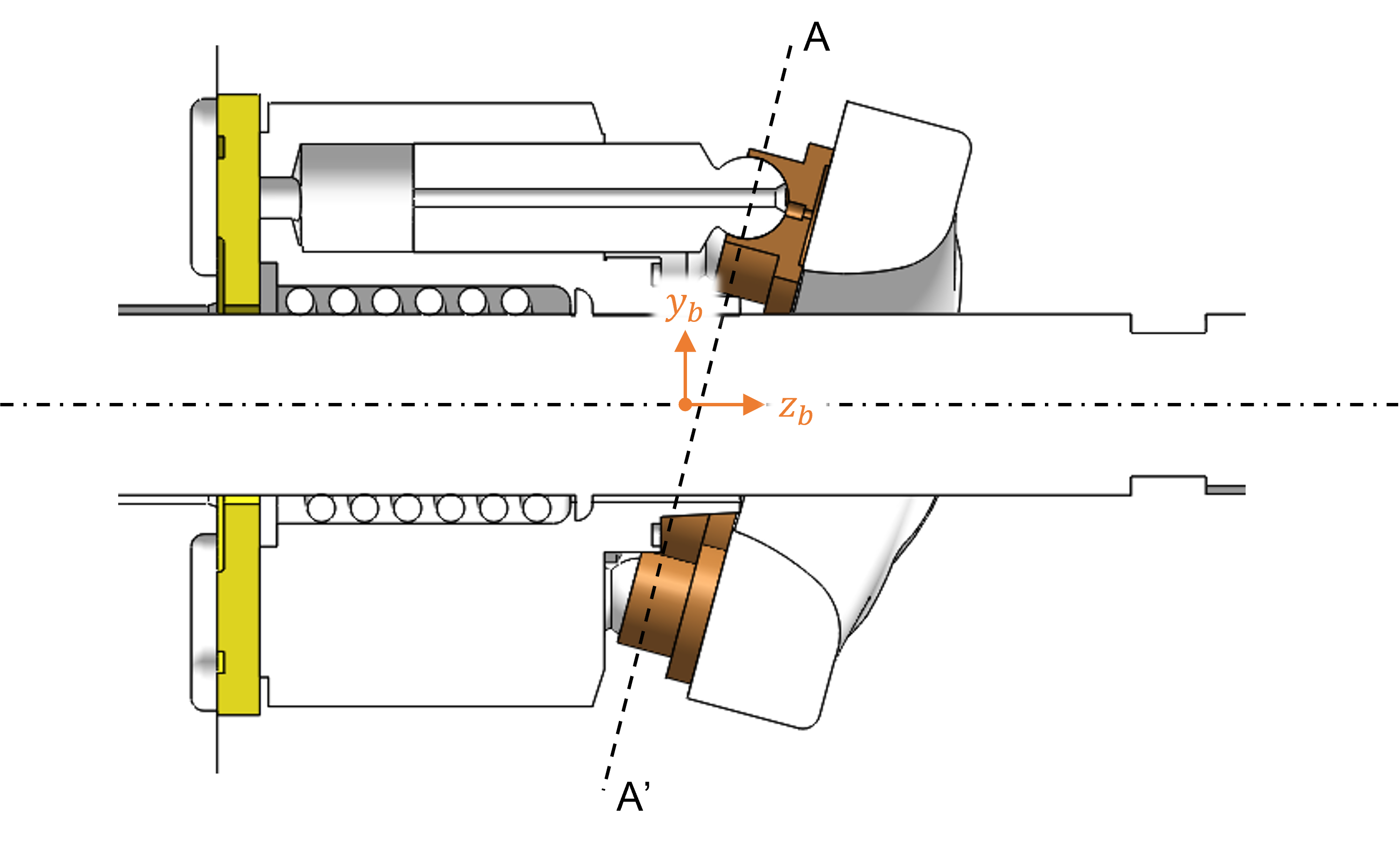
Cylinder Block

The cylinder body origin is defined at the crowning point or the point at which the shaft reaction acts such that the \(+z\) axis points towards the swashplate along the shaft axis. The other axis definitions follow the same convention as the global coordinate system. It is important to note that the block origin may or may not lie on the plane passing through the piston ball-joint centers.

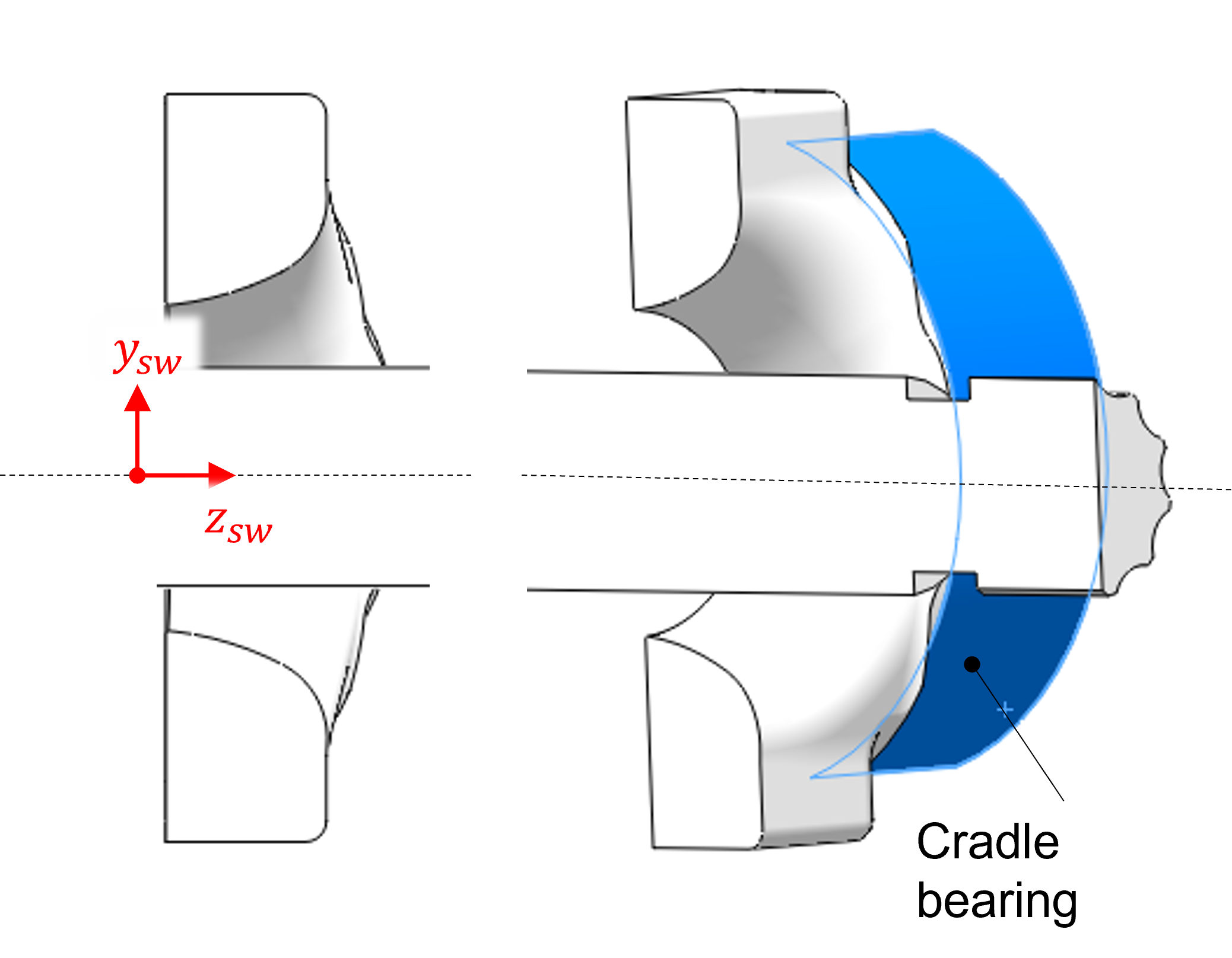
Swashplate

The swashplate origin lies at the swivel center of the swashplate on the shaft axes. The \(-z\) axis points in the direction of the cylinder block. The figure below represents the swashplate at zero displacement and summarizes the other axes which follow the right-hand rule.

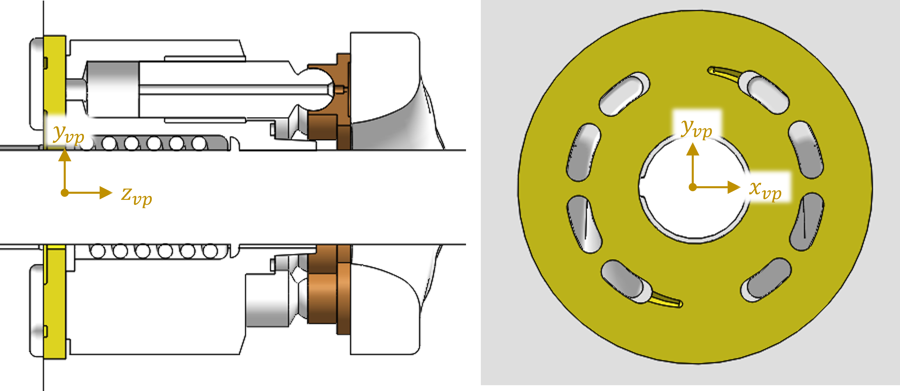
Valve Plate

The valve plate origin lies at the center of the running surface of the valve plate and on the shaft axes. The \(-z\) axis points in the direction of the cylinder block.

Film Coordinate System

The film coordinate systems are not required to be specified or assumed by the user in order to run the simulation. The template uses the geometric inputs specified to define these film origins internally.

Simulation Preprocessing Steps

Area File

Area files represents the area of the restriction between the displacement chamber and inlet/outlet ports for a complete rotation of the shaft. The restriction between the displacement chamber and the ports is modeled as an orifice of varying area in Multics.

To begin, follow the steps in the AVAS documentation to generate area files for the inlet and outlet ports.

Next, the area files from AVAS need to be converted to a format that Multics can read as a LookupTable. To perform this step, run the Utilities/make_area_file_APM.m script. The resulting output file should look similar to the sample below.

areaTable.txt

720 4
deg: 0 0.5
-: 1 1
mm^2: 0.661369       0.661369       ...    0.661369       0.661369
mm:   0.917649805    0.917649805    ...    0.917649805    0.917649805
mm^2: 0.48543        0.48543        ...    0.48543        0.48543
mm:   0.786173436    0.786173436    ...    0.786173436    0.786173436

This file’s structure follows the format described in the Lookup Table file section. Lines 1-3 describe the structure of the table – notice that the area file properties are given as a function of shaft angle. Lines 4 and 6 represent the orifice areas between displacement chamber and the inlet and outlet ports, respectively. Lines 5 and 7 represent the hydraulic diameter of the orifice between displacement chamber and the inlet and outlet ports, respectively.

The name of the area file is used as an input in the fileDict section of the inputDict.txt as shown below:

inputDict.txt

areaTable    ./common/areaTable.txt

Asperity Contact Polynomial Coefficients

Particularly during high-load, low-speed operation, solid body contact is common in APMs. Contact models that assume proportionality between the contact pressure and contact depth do not ensure a smooth transition between the hydrodynamic and mixed lubrication regimes. To avoid the resulting numerical issues associated, the Multics APM template by default uses a best-fit polynomial to smooth this transition.

For more details about asperity contact polynomials and how to generate polynomial coefficients, refer to the Asperity Contact Polynomial Coefficients page. Prior to setting up the APM tutorial simulation, make sure that you’ve followed the steps to generate an asperity contact polynomial, as this will be required later in the Polynomial Coefficients section of this tutorial.

Influence Matrix

Influence matrix deformation is a process described in other areas of the documentation. The algorithm assumes that deformation is elastic so that each node on the body will have a constant influence on all other nodes. Using these influences, a matrix is formed which can then be scaled by the pressure at each node to find the total deformation within the elements of the film.

To preprocess the influence matrices, ANSYS must be used to generate the meshes on each body. The process of initializing these bodies and running Influgen is covered here, so only the required named sets and boundary conditions will be elaborated on here. For all bodies, the coordinate system in ANSYS should be the same as that body’s coordinate system defined in the Body Coordinate Systems section above. If not, see the Body and IM Transformations section to perform the necessary coordinate transformations.

Cylinder Block

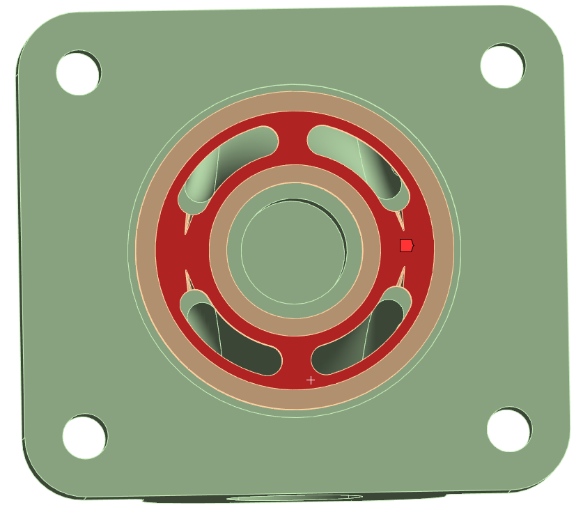
For the cylinder block, a total of 2n+1 named sets must be created, where n is the number of pistons in this pump.

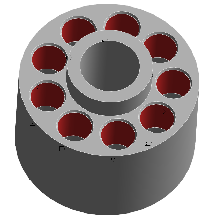
As seen above, each bore which forms a piston cylinder interface must be selected as a named set. Their names follow the convention pcX, where X is an integer and the number of the bore from 1 to n. The named set pc1 is aligned with the positive y axis of the body coordinate system and the rest are assigned increasingly in a counterclockwise order, looking from the swashplate to the valve plate.

Each displacement chamber must also be selected as a named set. Their names follow the convention dcX, where X follows the same conventions as for the cylinder bores.

Finally, the cylinder block valve plate film must be selected as a named set, as seen above, and renamed as cbvpfilm in ANSYS.

When generating the influence matrix for the cylinder block, inertia relief should be set to true, meaning that the constraint section of the input file should be left empty.

Piston

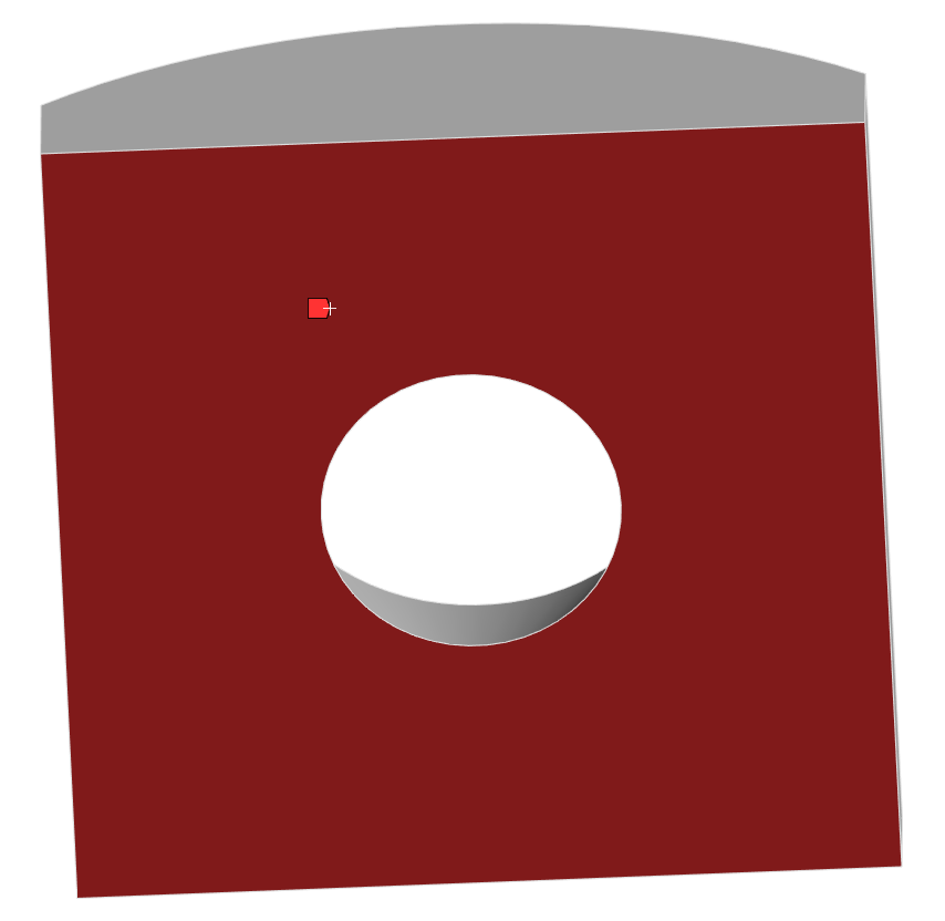
Four total named sets must be selected for the piston, the first of which is the running surface of the piston-cylinder interface, seen below.

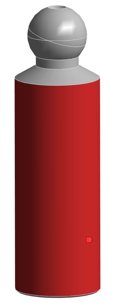
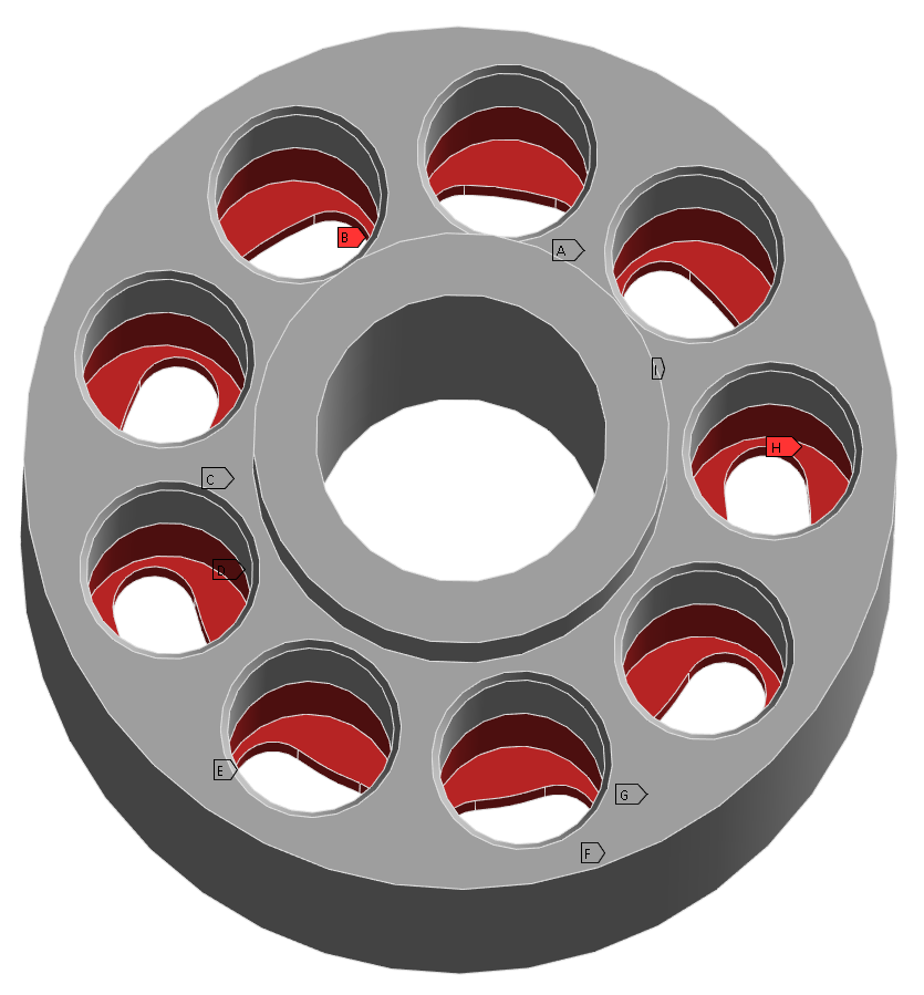
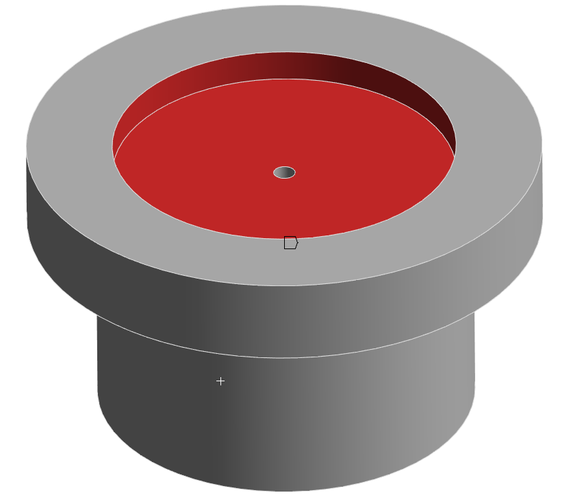
This set must be named cbpcfilm in ANSYS. The next set is the surfaces making up the displacement chamber, which is named dc. A figure of this is seen below.

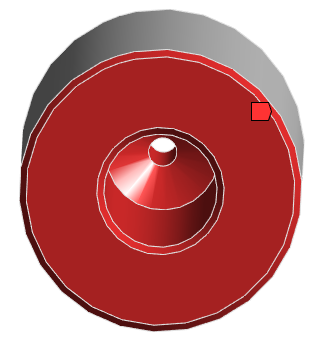
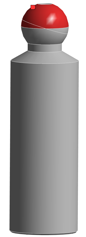
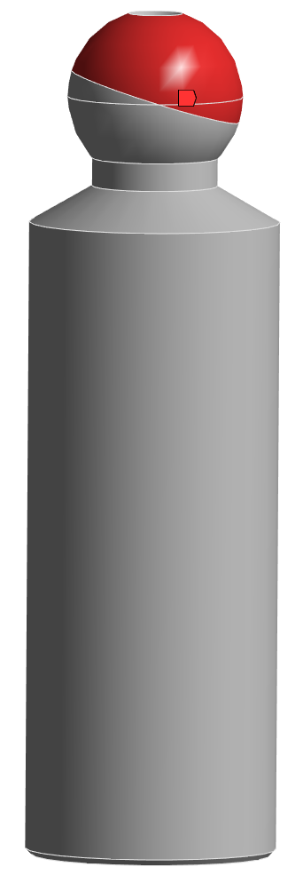
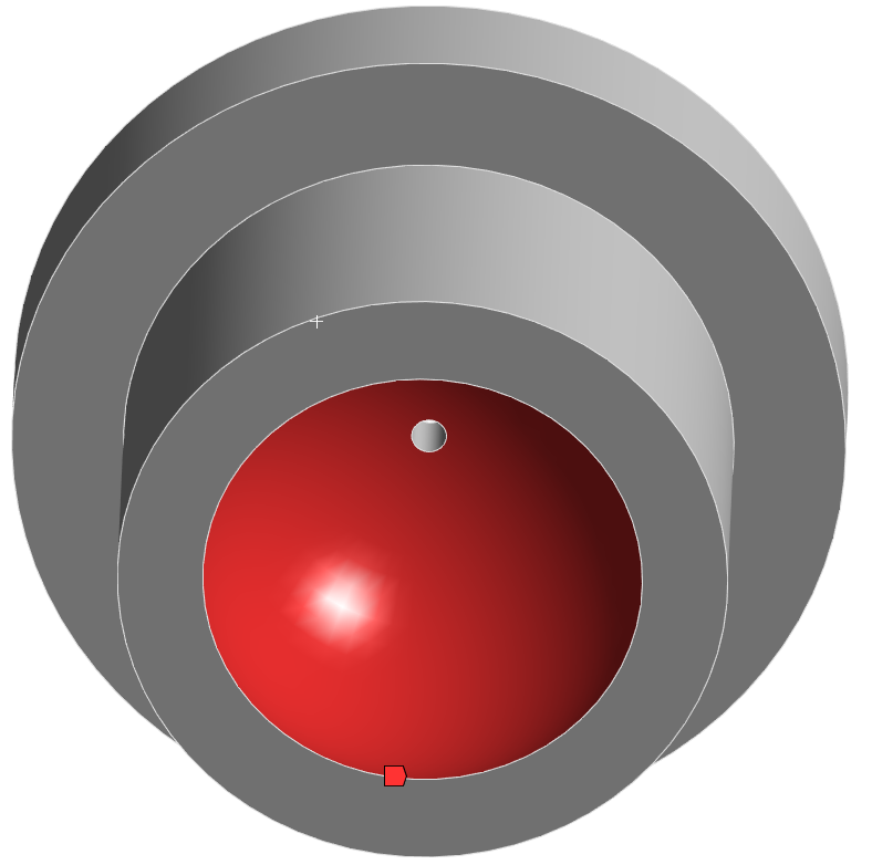
The final two sets are the areas of the piston ball covered by the slipper socket at zero and maximum displacement, called zerodisp and maxdisp respectively. These sets are used to calculate deformation based on the reaction force transferred through the ball socket. Figures of these two sets are seen below.

When generating the influence matrix for the piston, inertia relief should be set to true, meaning that the constraint section of the input file should be left empty.

Slipper

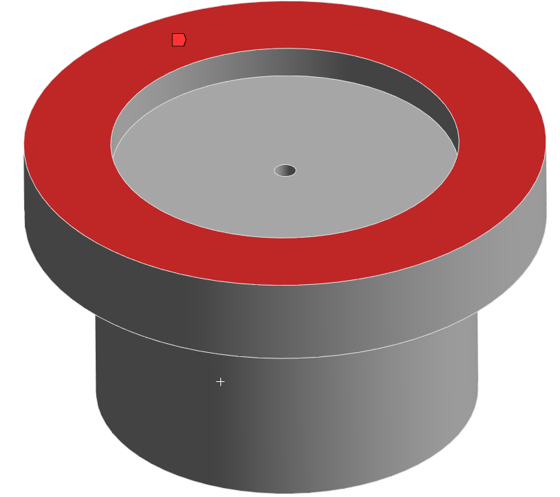
Three named sets are required to generate the influence matrices for the slipper. The first of these is the slipper pocket, which contains all surfaces touching fluid in the pocket. This set must be renamed pocket, and an example figure is seen below.

The second named set that must be created is the slipper socket, which must be renamed socket within ANSYS. These surfaces will have the same load applied to them as was on the piston ball.

The final named set needed is the running surface for the slipper-swashplate interface. This set must be named slspfilm and an example can be seen below.

When generating the influence matrix for the slipper, inertia relief should be set to true, meaning that the constraint section of the input file should be left empty.

Swashplate

Only two named sets must be selected to generate the swashplate influence matrices. The first of these is the slipper-swashplate interface running surface, which should be renamed slspfilm. Note that this surface should be selected so that it only contains the area that the slipper will run directly over. This will help reduce the file size. An example is seen below.

The other named set must contain the fixed surfaces of the swashplate. Often, this is a cradle bearing on the top surface. This named set does not require a specific name, but it must be remembered for the input file to Influgen. When generating the influence matrix for the swashplate, inertia relief should be set to false. Instead, the named set containing the fixed surfaces should be set as fixed in all directions in the input file to Influgen.

Valve Plate-End Case Assembly

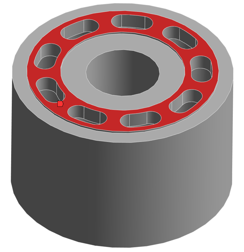
A total of four named sets must be created for the valve plate-end case assembly. Note that this influence matrix will have multiple bodies in the mesh. For instructions on how this should be done, reference the Influgen documentation page. The first set is the cylinder block-valve plate film, seen below.

This set must be renamed to cbvpfilm within ANSYS. The next two surface sets are the surfaces contained in the ports, one surface set for suction and one for delivery. The suction port should be named lp and the delivery port should be named hp. Take extra care when generating these surface sets to ensure that all surfaces encountering port pressure are selected. Examples of these are seen below.

For a symmetric pump, such as the one shown, the naming of these ports is not significant. For most pumps, the user must be careful to assign the correct pressure to its corresponding geometry. The final named set on this assembly does not have a required name, but, similar to the swashplate, its name must be remembered by the user for input to Influgen. This surface set will contain the surfaces on the end case which are fixed. Usually, these surfaces are where screws would be in a functioning pump.

When generating the influence matrix for the valve plate-end case assembly, inertia relief should be set to false. Instead, the named set containing the fixed surfaces should be set as fixed in all directions in the input file to Influgen. A template for the input.txt file that should be used can be seen below, where the pump and meshFile fields must be changed.

input.txt

// ------------------------- general informations -------------------------- //

section general

// analysis name
pump                 *Pump Name*
meshFile     *.cdb* File Path

// mesh dimension [m or mm]
dimension   mm

//Inertial relief
inrel       0

//ram
ram 16000

//Option to take only specified elsets. Default is all if this field not given
elsets 2 body1 body2

//command
//-botbody cbvpfilm -imgap -vtkset gap -imset hp -vtkset hp -imset lp -vtkset lp

endsection

// ------------------------------- Materials ------------------------------- //

section material

    name    bronze
    E       100e9   // [Pa]
    nu      0.3     // []
    rho     8500    // [kg/m^3]
    sets    1 body1 // volume sets using this material - VP
endsection

section material
    name    iron
    E       160e9   // [Pa]
    nu      0.3     // []
    rho     7000    // [kg/m^3]
    sets    1 body2 // volume sets using this material - Endcase

endsection

// ------------------------------- Constraint ------------------------------- //

section constraint

    // apply low pressure weld
    set FIX //set to apply to
    x 1 //fixed x
    y 1 //fixed y
    z 1 //fixed z

endsection

Body and IM Transformations

The generated STL bodies and IM can be moved in space by using a vector to specify the origin location from the default body origin and a corresponding transformation matrix.

Default Transformations

It is recommended the STL bodies to be printed and Influence Matrices generated be kept in the respective default body coordinate systems discussed in Body Coordinate System. In this case, the lubricating film locations will exactly be at the desired location with respect to the solid bodies printed. Similarly, the influence matrices generated such that the mesh is in the default coordinate system it would not require any further transformations. It is important to note that printing STL bodies is not mandatory but is recommended for better visualization as well as to ensure that all the bodies and films are in their respective desired positions. In this case all the rotation matrices as well as origin translations would be as follows:

inputDict.txt

unitConvVpEndCaseSTL    mm      [1; 0; 0; 0; 1; 0; 0; 0; 1]
rOrigVpEndCaseSTL       mm      [0; 0; 0]

unitConvVpEndCaseIM     m       [1; 0; 0; 0; 1; 0; 0; 0; 1]
rOrigVpEndCaseIM        m       [0; 0; 0]

Using Transformations

These transformations can also be used to shrink or change units of the STL bodies or the Influence Matrix files to be printed or used in appropriate units. Depending on the default unit settings of preprocessing tools used, the STL bodies and IM files may be in a different scale than the intended size of the pump. One such common instance of this is when the STL is generated without preserving the origin and unit of the CAD part (for e.g. Do not translate STL output to positive space option in SolidWorks ensures preserving of units and origin location). Similar discrepancies can happen in IM generation depending on the units in the mesh file CAD and the units specified in the input.txt in the IM folder.

The following example values of the transformation matrices can shrink the given STL body along all directions by 1000 times (correct meters to millimeters).

inputDict.txt

unitConvVpEndCaseSTL    m       [1e-3; 0; 0; 0; 1e-3; 0; 0; 0; 1e-3]
rOrigVpEndCaseSTL       m       [0; 0; 0]

However, these transformations can also be used to use STL bodies and IM generated in different coordinate systems by rotating, shrinking or translating to the default body origin used in the template.

APM Simulation Inputs

This section describes the inputs required for simulating an APM.

Operating Conditions

The main operating parameters of a conventional APM consist of the fluid pressure and temperature in the inlet/outlet ports, the fluid pressure and temperature in the case, the swashplate angle, and the operating speed of the APM. These operating conditions can be passed to Multics with the inputs summarized below:

pA

Pressure in the port on the \(+x\) axis. For a positive swashplate angle of the pump, this represents the outlet port of the pump

Unit: bar

TA

Temperature in the port on the \(+x\) axis. For a positive swashplate angle of the pump, this represents the outlet port of the pump

Unit: degC

pB

Pressure in the port on the \(-x\) axis. For a positive swashplate angle of the pump, this represents the inlet port of the pump

Unit: bar

TB

Temperature in the port on the \(-x\) axis. For a positive swashplate angle of the pump, this represents the inlet port of the pump

Unit: degC

pCase

Pressure in the casing of the pump

Unit: bar

TCase

Temperature in the casing of the pump

Unit: degC

betaMax

Maximum swashplate inclination angle for the given operating condition. It is important to note that the sign of this input will change the inlet and outlet port definition for a given coordinate system

Unit: deg

beta

Swashplate inclination angle for the given operating condition. For a fixed displacement unit, this value will be equal to betaMax. It is important to note that the sign of this input will change the inlet and outlet port definition for a given coordinate system

Unit: deg

omega

Operating speed of the machine. This value needs to be in accordance to the \(z\)-axis of the coordinate system. The value needs to be negative for pumping mode of operation provided the swashplate angle is positive

Unit: rev/min

The following table summarizes a few cases explaining the use of the above parameters to appropriately define the APM operation to be simulated

APMoperation.txt

Case 1:
pA      pB      beta    betaMax         omega       Operation
200     20      15          20                  2000        Pumping mode at 75% displacement
Case 2:
pA      pB      beta    betaMax         omega       Operation
200     20      -20     20          2000        Motoring mode with 100% displacement
Case 3:
pA      pB      beta    betaMax         omega       Operation
200     20      15      20          -2000       Motoring mode with 75% displacement

Simulation Options

The APM template allows a significant degree of customization. Using the same template code, a wide variety of APM geometries can be simulated, and users can toggle physical and numerical calculations such that the fidelity of the simulation matches their needs. This section describes the various simulation options available when simulating the APM.

General Options

nRev

Number of revolutions to run the simulation model.

Unit: -

fluidType

Fluid property type

• 0 - Fluid Props Sub/Super with cavitation integrated in files

• 1 - Single fluid props super with cavitation specified

• 2 - User expression with cavitation specified

Unit: -

degPrint

Print interval to report results. Recommended upper limit 1 deg.

Unit: deg

Lubricating Interface Selection

The following options allows to selectively solve for different lubricating interfaces based on a binary input. Note that these switches will change the number of films to be solved together with the lumped parameter model depending on the combination of these three inputs.

The following input values are valid for the options in this section:

Input Value	Description
1	Solve Reynolds equation for film
0	Use analytical model to approximate film

isBlockFilm

Switch to select whether to solve for the cylinder block/valve plate interface simulation

Unit: -

isPistonFilm

Switch to select whether to solve for the piston/cylinder interface simulation

Unit: -

isSlipperFilm

Switch to select whether to solve for the slipper/swashplate interface simulation

Unit: -

For example, setting isPistonFilm and isSlipperFilm simultaneously equal to 1 will run a single piston/cylinder interface coupled with a slipper/swashplate interface along with a lumped-parameter model. Setting all the three films simultaneously equal to 1 will solve for all the interfaces in the APM simulation (e.g. 19 films for a 9-piston APM).

Mixed Lubrication

The following options allow the user to select whether mixed lubrication is solved for or not in the film. These inputs are ignored if not solving the Reynolds equation for the film (i.e., if the corresponding input in the Lubricating Interface Selection section is 0).

The following input values are valid for the options in this section:

Input Value	Description
1	Mixed lubrication is considered
0	Mixed lubrication is not considered

isMixedLubBlockFilm

Switch to select whether to consider mixed lubrication in the cylinder block/valve plate interface simulation

Unit: -

isMixedLubPistonFilm

Switch to select whether to consider mixed lubrication in the piston/cylinder interface simulation

Unit: -

isMixedLubSlipperFilm

Switch to select whether to consider mixed lubrication in the slipper/swashplate interface simulation

Unit: -

Pressure Deformation

The following options allow the user to select the structural deformation model to be used while solving the film. These inputs are ignored if not solving the Reynolds equation for the film (i.e., if the corresponding input in the Lubricating Interface Selection section is 0).

The following input values are valid for the options in this section:

Input Value	Description
0	No deformation
1	Analytical micro deformation
2	Influence matrix deformation

Note: If the influence matrix deformation is selected additional files are required as input in the fileDict option, which will be discussed in the IM Preprocessing section.

isDefBlockFilm

Switch to select deformation model in the cylinder block/valve plate interface simulation

Unit: -

isDefPistonFilm

Switch to select deformation model in the piston/cylinder interface simulation

Unit: -

isDefSlipperFilm

Switch to select deformation model in the slipper/swashplate interface simulation

Unit: -

Wear Profile

The following options allow the user to add an artificial measured wear profile on solid parts forming the lubricating film. For example, a wear profile can be added to the cylinder bore and piston of the piston/cylinder interface, or the slipper body of the slipper/swashplate interface.

The following input values are valid for the options in this section:

Input Value	Description
1	Measured wear profile is provided in the fileDict
0	No measured wear profile is simulated

isBoreProfile

Switch to select whether a surface profile is selected for the cylinder bore

Unit: -

isPistonProfile

Switch to select whether a surface profile is selected for the piston

Unit: -

isSlipperProfile

Switch to select whether a surface profile is selected for the slipper

Unit: -

Film Parameters

The following parameters define the parameters of the lubricating films of the APM.

nPtsBlockFilm

Number of points in the cylinder block/valve plate lubricating film mesh. Recommended starting value of \(12500\)

Unit: -

nPtsPistonFilm

Number of points in the piston/cylinder lubricating film mesh. Recommended starting value of \(5000\)

Unit: -

nPtsSlipperFilm

Number of points in the slipper/swashplate lubricating film mesh. Recommended starting value of \(5000\)

Unit: -

hInitBlockFilm

Initial film thickness for the cylinder block/valve plate lubricating film. Recommended starting value of \(10\ \mu m\)

Unit: micron

hInitPistonFilm

Initial film thickness for the piston/cylinder lubricating film. Recommended starting value of \(10\ \mu m\)

Unit: micron

hInitSlipperFilm

Initial film thickness for the slipper/swashplate lubricating film. Recommended starting value of \(10\ \mu m\)

Unit: micron

Numerical Parameters and Relaxation

The following section represents the different inputs to define the time stepping while solving for lubricating films (applicable when at least one lubricating film is enabled in Lubricating Interface Selection). Although there are recommended starting values, these values vary from case to case. Therefore, it is recommended to observe the individual time steps in the simulation results to determine suitable changes in the values.

maxCFL

Maximum CFL (Courant-Friedrichs-Lewy condition) number for lubricating films. Recommended starting value of 10

Unit: -

squeezeLimiter

Maximum percent change in gap height in a single time step. Note that this value is scaled with the initial clearance of the interface defined in the Film Parameters. Recommended starting value of 0.5%.

Unit: %

impContr

Upper threshold change in the Reynolds equation solution by a small perturbation of density in the perturbed universal Reynolds equation. Recommended value of 10%. If this value is crossed, the impedance effects will shrink the Reynolds time step.

Unit: %

impContrHard

Hard threshold change in the Reynolds equation solution by a small perturbation of density in the perturbed universal Reynolds equation. Recommended value of 50%. If this value is exceeded, both the impedance contribution as well as the Reynolds time step are shrunk.

Unit: %

impShrinkRate

Defines the rate by which the impedance time step shrinks due to impedance contributions exceeding the thresholds. Recommended value of 0.75.

Unit: -

filmStepMaxGrowth

Maximum percent change in the Reynolds integrator time step from the previous time step. Recommended starting value of 25%. Note that this time step is different than the simulation time printed at each print interval.

Unit: %

IntegratorMaxSteps

Maximum steps for the integrator. Recommended value of \(10^8\)

Unit: -

IntegratorAbsTol

Absolute tolerance for convergence. Recommended value of \(10^{-8}\)

Unit: -

IntegratorRelTol

Relative tolerance for convergence. Recommended value of \(10^{-8}\)

Unit: -

ompNthreads

Number of threads for parallel implementation. Recommended value depends on the computer. Parallel computations will speed up simulations significantly.

Unit: -

Polynomial Coefficients

To accurately simulate mixed and boundary lubrication, an asperity contact polynomial should be fit and provided to Multics as discussed in the Asperity Contact Polynomial Coefficients section.

The APM object accepts polynomial coefficients of any degree, provided as an array of numbers to the polyCoeffsBlockFilm input in the inputDict.txt. An n-order polynomial fit will have n+1 coefficients. The asperity contact polynomial will be used for all lubricating interfaces (piston-cylinder, cylinder block-valve block, slipper-swashplate).

Example: Suppose that we follow the instructions in the Asperity Contact Polynomial Coefficients section and generate the following ninth-order asperity contact polynomial:

Linear model Poly9:
f(x) = p1*x^9 + p2*x^8 + p3*x^7 + p4*x^6 +
       p5*x^5 + p6*x^4 + p7*x^3 + p8*x^2 + p9*x + p10
Coefficients (with 95% confidence bounds):
p1 =   -6.66e-05  (-6.775e-05, -6.546e-05)
p2 =   -0.001535  (-0.001562, -0.001508)
p3 =     -0.0143  (-0.01457, -0.01404)
p4 =     -0.0684  (-0.06978, -0.06701)
p5 =     -0.1764  (-0.1806, -0.1723)
p6 =     -0.2415  (-0.2488, -0.2343)
p7 =     -0.1753  (-0.1822, -0.1685)
p8 =     -0.0156  (-0.01878, -0.01242)
p9 =     -0.1972  (-0.1978, -0.1966)
p10 =     0.07652  (0.07646, 0.07659)

Goodness of fit:
SSE: 0.0002519
R-square: 1
Adjusted R-square: 1
RMSE: 0.0005044

To provide these polynomial coefficients to the APM model, add the following line to the inputDict.txt:

polyCoeffsBlockFilm   -   [-6.66e-05; -0.001535; -0.0143; -0.0684; -0.1764; -0.2415; -0.1753; -0.0156; -0.1972; 0.07652]

Geometry Inputs

The following section describes the geometry inputs of the hydraulic unit.

nPiston

Number of pistons or displacement chambers in the APM

Unit: -

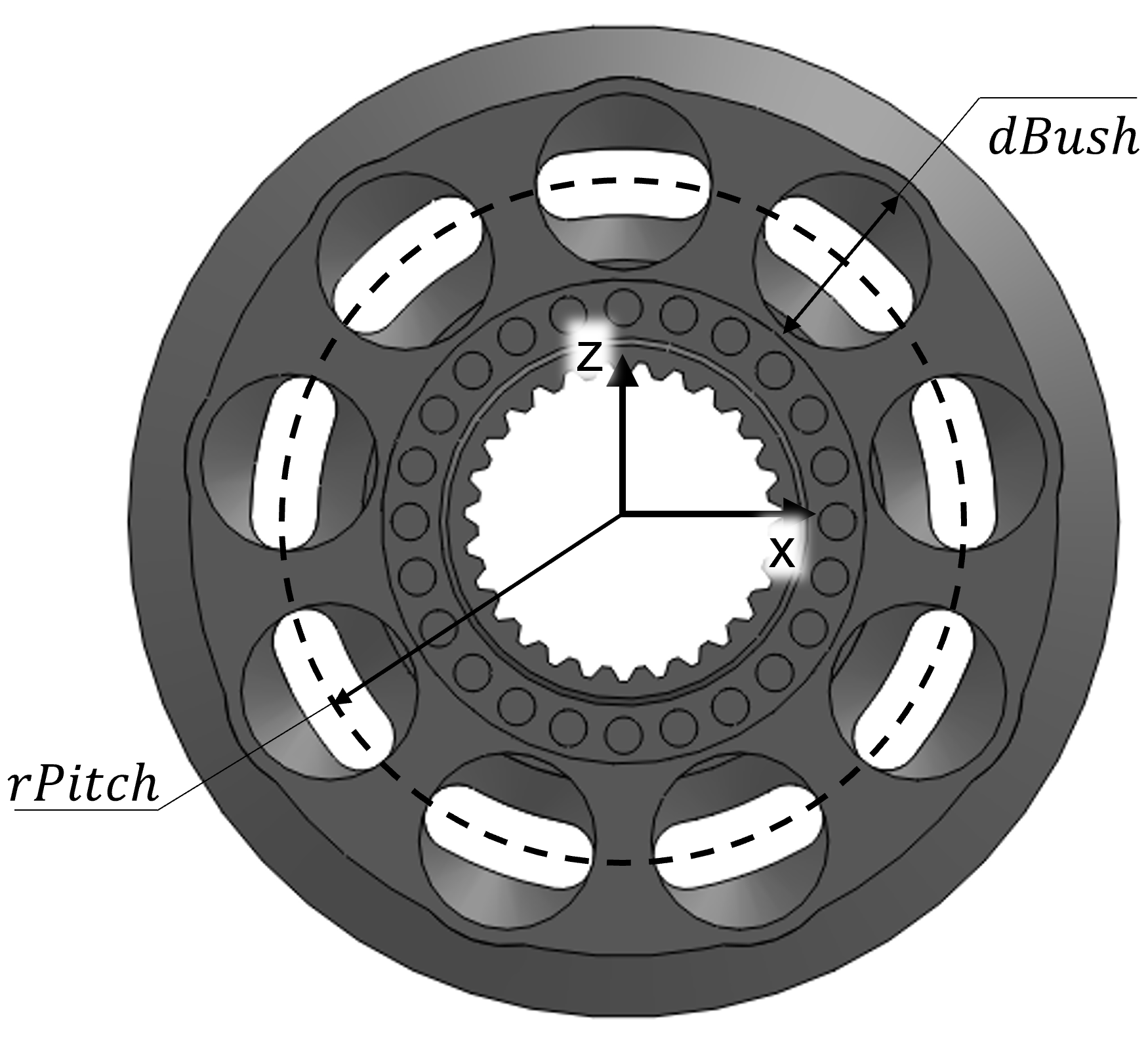
dPitch

Pitch diameter. The diameter of the circle passing through the centers of the cylinder bores in the cylinder block of the APM as seen in the figure.

Unit: mm

dBore

Diameter of the cylinder bore. For APM with a separate bushing insert, this value needs to consider the inner diameter of the bushing insert.

Unit: mm

dPiston

Outer diameter of the piston surface forming the piston/cylinder interface

Unit: mm

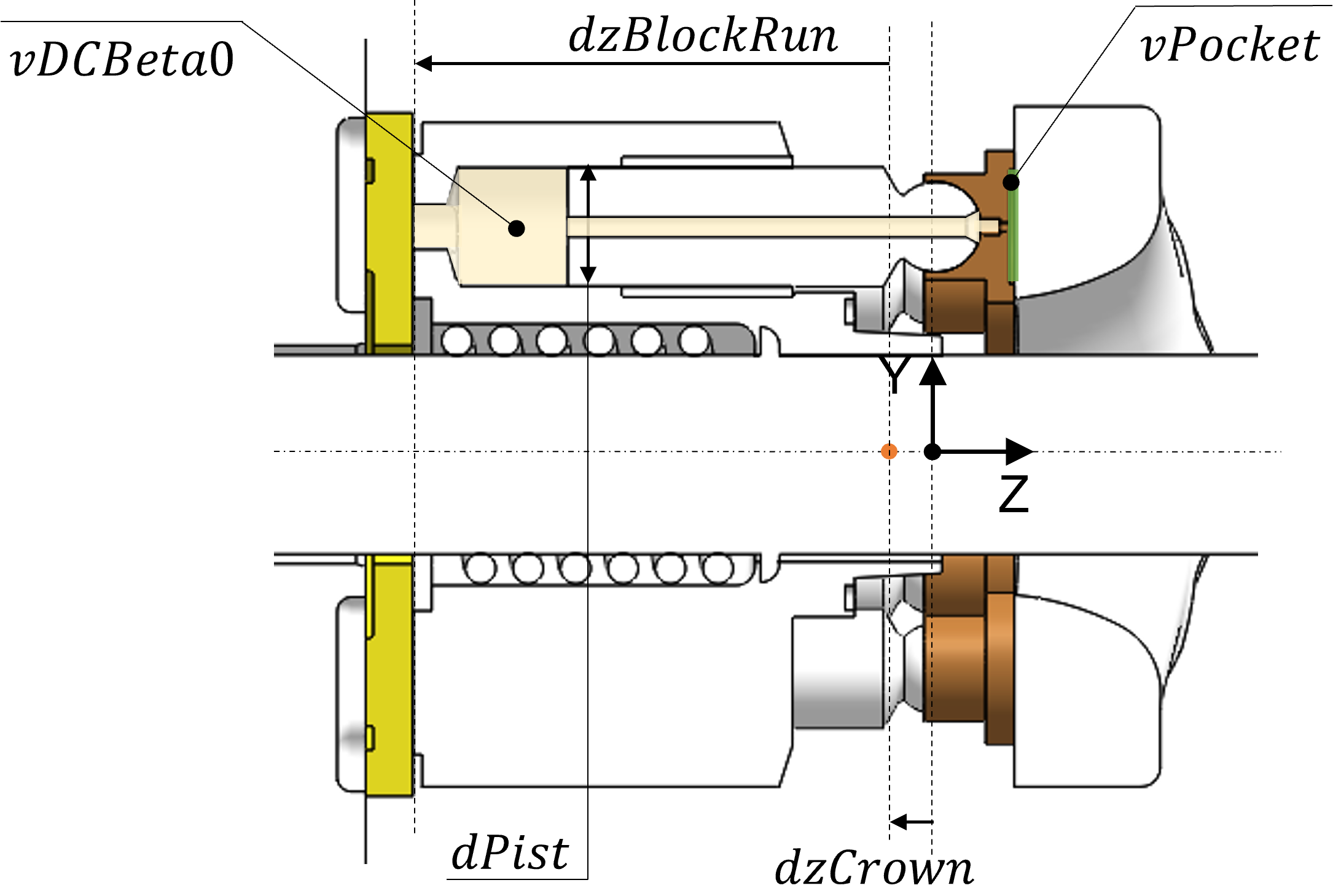
dzCrown

Distance of the shaft reaction point/block body origin from the global origin of the APM template along the \(z\) axis. A positive dzCrown means the crowning point shifted towards the swashplate from the ideal crowning point.

Unit: mm

dzBlockRun

Distance of the cylinder block running surface of the cylinder block-valve plate lubricating film from the block body origin along the \(z\) axis

Unit: mm

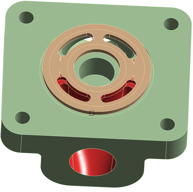
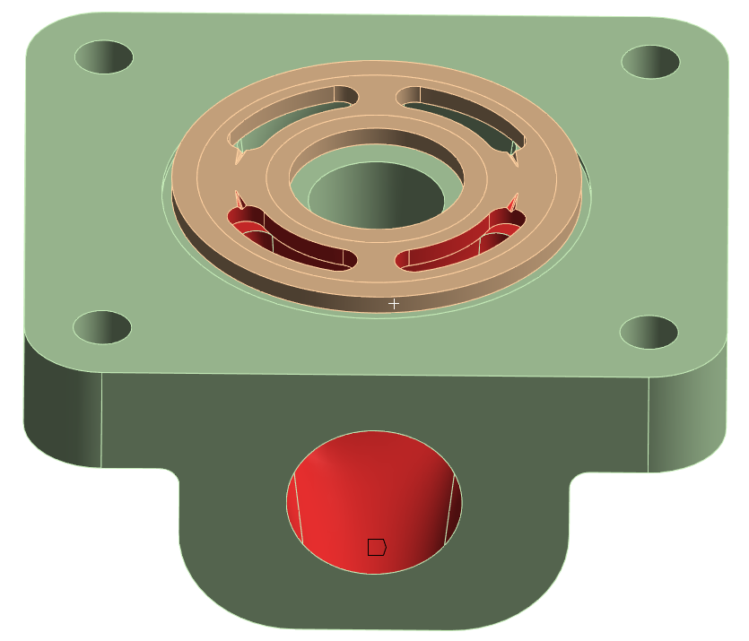
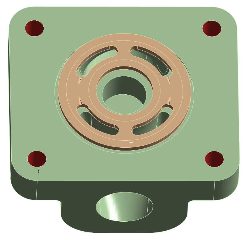
vPocket

Fluid volume enclosed in the slipper pocket (as highlighted in green)

Unit: mm^3

vDCBeta0

Displacement chamber volume at zero displacement (as highlighted in beige). Note that the extent of volume to be considered in the piston and slipper bodies as the displacement chamber volume varies from case to case.

Unit: m^3

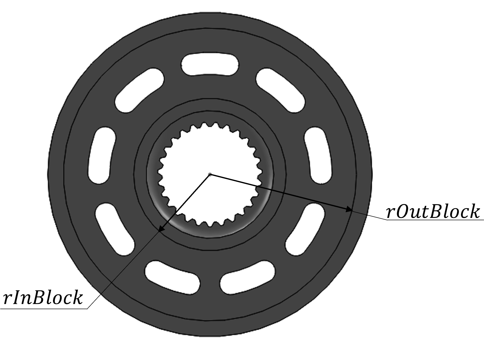
dInBlock

Inner diameter of the cylinder block running surface forming the cylinder block-valve plate lubricating interface

Unit: mm

dOutBlock

Outer diameter of the cylinder block running surface forming the cylinder block-valve plate lubricating interface

Unit: mm

FSpringBlock

Cylinder block spring force. This input typically comes from the pump manufacturer.

Unit: N

FSlipperHoldDown

Slipper hold down force applied on a single slipper. This input typically comes from the pump manufacturer. If simulating a fixed hold down, this value can be zero.

Unit: N

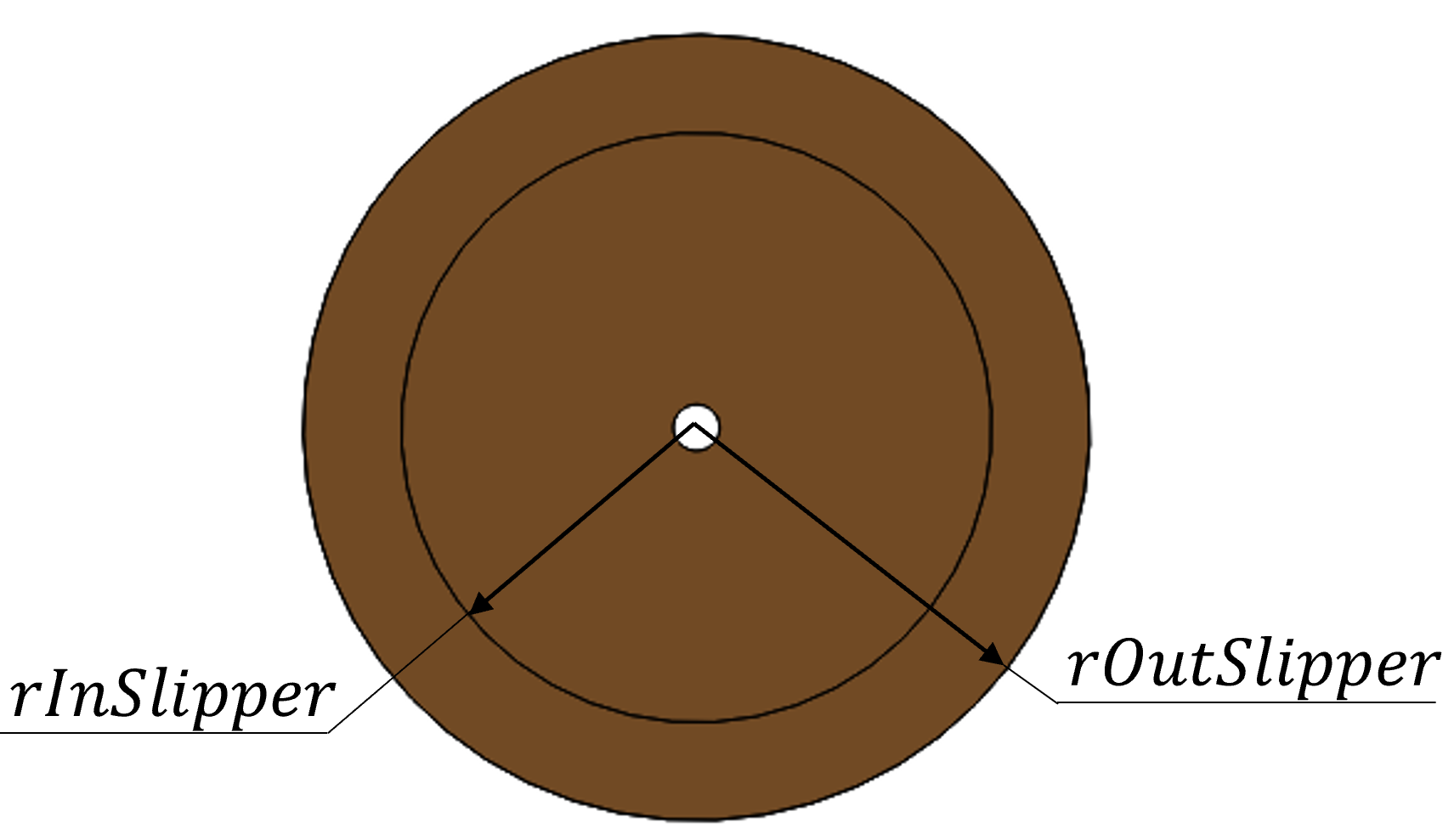
dInSlipper

Inner diameter of the slipper running surface forming the slipper/swashplate lubricating interface

Unit: mm

dOutSlipper

Outer diameter of the slipper running surface forming the slipper/swashplate lubricating interface

Unit: mm

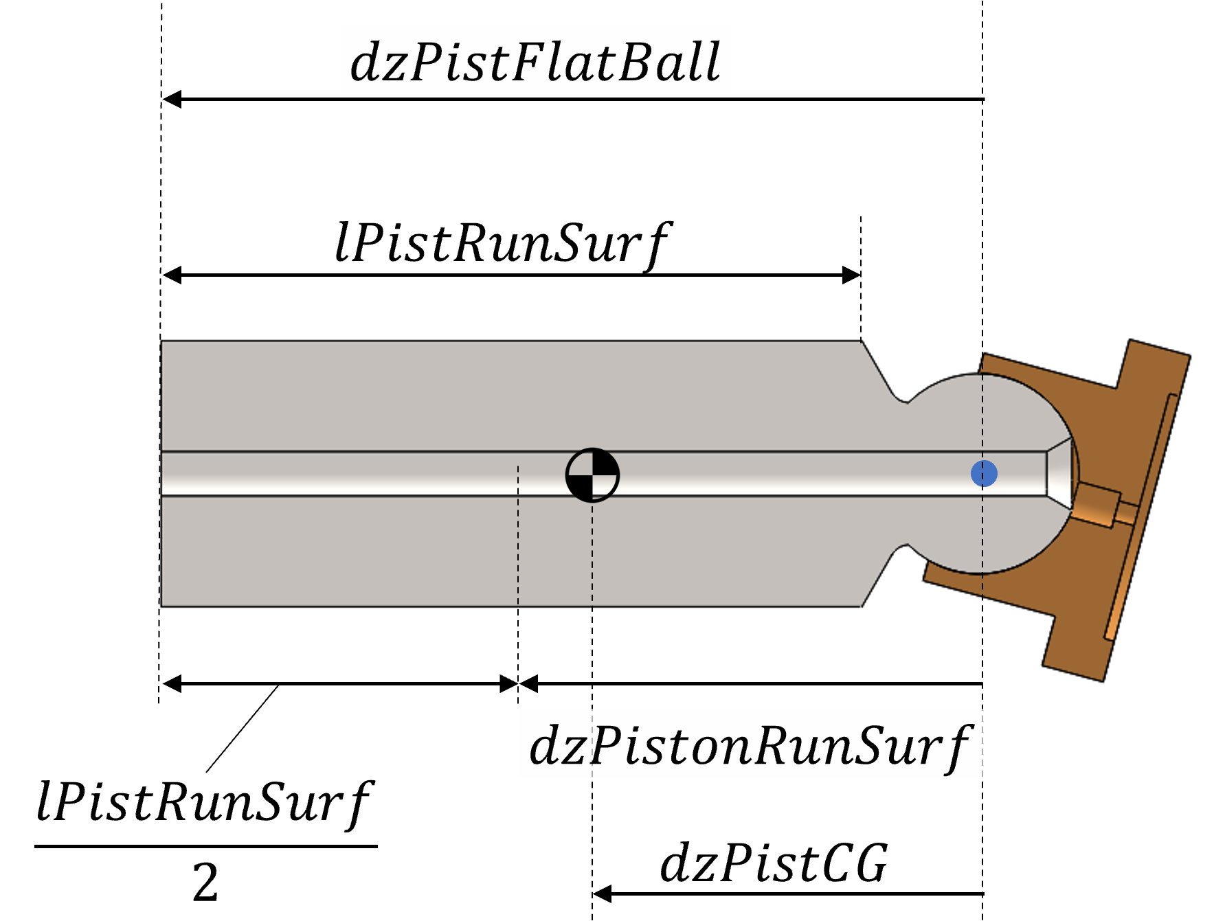
lPistonRunSurf

Piston running surface length

Unit: mm

dzPistonRunSurf

Distance of piston running surface center from piston ball head center/piston body origin (positive sense from valve plate to swashplate)

Unit: mm

dzPistonCG

Distance of piston body center of gravity from piston ball head center/piston body origin (positive sense from valve plate to swashplate)

Unit: mm

dzPistonFlatBall

Distance of flat end of the piston from piston ball head center/piston body origin (positive sense from valve plate to swashplate)

Unit: mm

rSocket

Radius of the slipper socket

Unit: mm

pocketOrifDia

Pocket orifice diameter. This should be the minimum diameter that will connect the displacement chamber to the pocket and its location can vary with specific pump design.

Unit: mm

dzSlipCG

Distance of slipper body center of gravity from slipper socket center/slipper body origin (positive sense from valve plate to swashplate)

Unit: mm

dzSlipRun

Distance of slipper running surface from slipper socket center/slipper body origin (positive sense from valve plate to swashplate)

Unit: mm

lBoreRunSurf

Cylinder block bore running surface length possible

Unit: mm

dzBushingRunSurf

Distance of the bushing running surface center on block from the cylinder block body origin along the \(z\) axis

Unit: mm

dzBlockCG

Distance of ideal crowning point to the center of gravity of the block to the cylinder block origin

Unit: mm

For the case of APM with an bushing insert typically of a softer material, the similar parameters can be revised to account for the actual length of the bushing as shown in the figure below.

For a bushing insert with an undercut, do not consider the portion of the bushing with the undercut for the above geometry parameters.

Material Properties

Inertial Properties

Analyzing Results

Plotting Results

Analyzing Lumped Parameter Results

Analyzing Film Properties